| Issue |
Knowl. Manag. Aquat. Ecosyst.
Number 426, 2025
Biological conservation, ecosystems restoration and ecological engineering
|
|
|---|---|---|
| Article Number | 3 | |
| Number of page(s) | 14 | |
| DOI | https://doi.org/10.1051/kmae/2024025 | |
| Published online | 15 January 2025 | |
Research Paper
An evaluation of artificial floating littoral zones to support fish communities in reservoirs
1
INRAE, Aix Marseille Univ, RECOVER, 3275 Route Cézanne, 13100 Aix-en-Provence, France
2
Pôle R&D Ecosystèmes Lacustres (ECLA), OFB-INRAE-USMB, Aix-en-Provence, France
3
ECOCEAN, 1342 Avenue de Toulouse, 34070 Montpellier, France
4
OFB, Service ECOAQUA, DRAS, 3275 Route Cézanne, 13100 Aix-en-Provence, France
* Corresponding author: This email address is being protected from spambots. You need JavaScript enabled to view it.
Received:
27
August
2024
Accepted:
16
December
2024
Abstract
Artificial water level fluctuations (WLF) in reservoirs impact fish communities by degrading littoral habitats. To mitigate these negative effects, artificial floating islands that mimic natural littoral zones appear as a promising mitigation tool. However, their effectiveness in supporting fish communities remains poorly documented. In this study, three artificial floating littoral zones (FLOLIZ, 70 m2 surface area) were installed in a French hydropower reservoir subject to extreme WLF. Fish communities were assessed in spring and summer over four years in FLOLIZ and in control littoral stations during daytime and nighttime. Fish, especially juveniles, did not appear more frequently in FLOLIZ than in control littoral stations during daytime. At night, both adult and juvenile fish were more abundant in the littoral zone of the reservoir. During the day, the fish community in FLOLIZ was mainly composed of juvenile Chondrostoma toxostoma and adult Perca fluviatilis. Differences occurred only for a few species and life stages (juvenile vs adult); however, in general, results indicated greater abundance or richness in control littoral stations. These results do not support the effectiveness of FLOLIZ in mitigating deleterious effects of artificial WFL. The distance of FLOLIZ to the littoral zone could explain these results. Further studies in different environmental conditions, in different ecosystems and with different FLOLIZ designs are needed to provide additional information on the effectiveness of such structures as a mitigation tool.
Key words: Artificial floating island (AFI) / ecological engineering / water level fluctuations (WLF) / mitigation / fish habitat
© Q. Salmon et al., Published by EDP Sciences 2025
 This is an Open Access article distributed under the terms of the Creative Commons Attribution License CC-BY-ND (https://creativecommons.org/licenses/by-nd/4.0/), which permits unrestricted use, distribution, and reproduction in any medium, provided the original work is properly cited. If you remix, transform, or build upon the material, you may not distribute the modified material.
1 Introduction
At the interface between aquatic and terrestrial ecosystems, the littoral zone of lakes offers complex and valuable habitats for biodiversity and plays a major role in their overall functioning (Sala and Güde, 2006; Czarnecka, 2016; Meerhoff and de los Ángeles González-Sagrario, 2022). Specifically, it hosts numerous fish species, at least at some life stages, in which they can feed, grow, shelter, and spawn (Winfield, 2004; Říha et al., 2011). Water level fluctuations (WLF), depending on the hydrological regime, control the structure and functioning of littoral zones (Sutela et al., 2013; Zohary and Gasith, 2014; Evtimova and Donohue, 2016). In reservoirs, WLF can be extreme in amplitude and frequency (Coops et al., 2003; Hirsch et al., 2014), leading to an homogenization and impoverishment of littoral habitats (Furey et al., 2004; Logez et al., 2016). This has cascading negative effects on fish communities (Leira and Cantonati, 2008).
Although fish are often mobile enough to follow WLF, the loss or inaccessibility of littoral habitats can impact their behavior, survival, growth, spawning, and recruitment (Carmignani et al., 2019). For example, artificial WLF reduce the abundance and modify the assemblage of benthic invertebrates, which can decrease insectivorous fish density and diversity or limit the growth of young-of-year (YOY) in some species (Haxton and Findlay, 2009; Sutela et al., 2011; McDowell, 2012). The scarcity of preferred habitats can lead to increased intraspecific competition, which causes smaller individuals to migrate to deeper areas (Fischer and Öhl, 2005). For species that spawn in the littoral zone (e.g. phytophilous species), a lack of suitable habitats during the spawning period can lead to poor recruitment and population decline (Wegener and Williams, 1975; Farrell, 2001). A significant drawdown leading to shoreline exposure and egg desiccation after spawning can significantly reduce or even totally suppress recruitment (Grabowski and Isely, 2007; Kahl et al., 2008). In addition, fish populations can decline because of a lack of shelter that exposes YOY to predation (Wolcox and Meeker, 1992). These deleterious effects have led both researchers and managers to look for mitigation solutions to WLF (Trussart et al., 2002; Tundisi and Matsumura-Tundisi, 2003).
The control of WLF when the littoral zone is the most intensively used by fish (e.g. spring for spawning) (Westrelin et al., 2022; Maday et al., 2023) often conflicts with the uses of reservoirs and is difficult to implement. Consequently, ecological engineering methods using artificial habitats have been widely studied and their effectiveness to enhance fish habitats has been shown (Zalewski and Frankiewicz, 2002; Pedicillo et al., 2008; Santos et al., 2008). However, the attractiveness of these artificial habitats differs according to various parameters (depth, temperature, diel cycle) (Walters et al., 1991; Moring and Nicholson, 1994). Moreover, most studies were carried out in lakes with low WLF of a few meters. Santos et al. (2011) tested littoral artificial habitats in a reservoir with relatively high WLF (around 8 m) and needed to move the habitats several times to keep them immersed. The authors concluded that self-adapting habitats would be much more effective. This is the case of artificial floating islands (AFI), which consist of floating frames covered with plants, available for aquatic fauna no matter the WLF. These one-dimensional floating structures have been widely used in Europe and Asia for aesthetic purposes, for water quality improvement, and for habitat enhancement (Nakamura and Mueller, 2008; Yeh et al., 2015). By providing new and complex substrates, AFI concentrate significant aquatic biodiversity (Prashant and Billore, 2020; Salmon et al., 2022) and were also used as a mitigation tool to sustain fish populations by providing spawning habitats (Nakayama, 1986 in Nakamura and Mueller, 2008; Gillet, 1989). Recently, two studies again highlighted their potential to support juvenile fish (Huang et al., 2017; De Moraes et al., 2023). However, these studies remain few in number and have been carried out over short periods. Additionally, the structures used were mainly designed to support spawning and not to provide refuge and nursery habitats for fish.
In this study, we designed an innovative artificial floating island named Floating Littoral Zones (FLOLIZ) that mimics a natural littoral zone. It is a three-dimensional structure with subaquatic stages, two types of mineral substrate, helophyte and hydrophyte plants. Three FLOLIZ have been installed in a French hydropower reservoir subject to extreme WLF (up to 50m) and studied over four years. We aimed at assessing their effectiveness as new functional habitats to support fish communities. We hypothesized that fish abundance and species richness would be higher in FLOLIZ than in control stations due to the diversity and complexity of that habitats and their availability at any water level. We expected this pattern would be particularly enhanced in spring and summer, compared to low activity seasons. Finally, we expected that the fish assemblage would differ between FLOLIZ and control stations due to significant differences in the habitats. Specifically, we expected a higher abundance of vegetation-dependent species in FLOLIZ.
2 Materials and methods
More details on the study site, FLOLIZ design and sampling stations can be found in Salmon et al. (2022).
2.1 Study site
The study was conducted in Serre-Ponçon reservoir located in South-Eastern France (44.5117°N; 6.3326°E) (Fig. 1A). This is one of the largest reservoirs in Metropolitan France, with a surface area of 28 km2 (20 km long and 3 km wide at the maximum), a volume of 1272 km3 at a maximum altitude of 780 m and a maximum depth of about 110 m. The dam was built in 1959 to produce hydropower. The reservoir is also used to control flooding by the two main inflow rivers (Durance and Ubaye) and to supply irrigation and drinking water needs. These uses lead to extreme WLF up to 49 m (27 m in average over 2018–2022) (Data from Electricité de France, French Electrical Company). The fluctuations are seasonal, with a significant decrease in water level between early autumn and late winter, and a significant rise in spring following the snowmelt (Fig. A1 in Appendix). The daily amplitude of WLF can reach 1.6 m (Data from Electricité de France). In summer, the water level is kept stable at a high level for recreational activities (altitude 780 m). These extreme WLF prevent littoral vegetation from growing and lead to morphological alterations on the banks. Serre-Ponçon is a monomictic reservoir, with stratification occurring from March to September. The latest monitoring of Serre-Ponçon’s water quality as part of the Water Framework Directive (WFD; 2000/60/EC), concluded that it had good water quality with an oligo-mesotrophic status (Data 2022 from WFD).
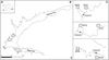 |
Fig. 1 Location of FLOLIZ and control stations in Serre-Ponçon hydropower reservoir. (A) Location of Serre-Ponçon hydropower reservoir in France; (B) Reservoir contour at the highest water level (altitude 780 m) and location of 3 sampling zones (ellipses); (C) Focus on the 3 zones (suffixed 1, 2 and 3) with control stations and FLOLIZ. DCS: Distant Control Station, NCS: Nearby Control Station, FLOLIZ: Floating Littoral Zone. |
2.2 FLOLIZ design
FLOLIZ are 14 m long and 5 m wide. The floating part is composed of high-density polyethylene (HDPE) caissons (Fig. 2A). One caisson out of two contains clods of soil with local helophyte plants such as Phragmites australis, Calamagrostis epigeois, Salix sp, and Carex elaya (Fig. 2B). The submerged part is made of three extruded aluminium structures (4 m wide × 4 m long); the central one is 1 m deep and the two others are 0.5 m deep. These different underwater levels mimic a natural littoral zone. The aluminium structures are tied to the floating caissons by steel chains. The bottom and two sides of these structures are covered with steel mesh cages (0.5 × 0.8 × 0.25 m) filled with inert, non-pollutant substrates (cellular glass stone, recycled oyster shells) to simulate a mineral soil. The mesh cages on both sides partly protect the inner area from waves and currents. Empty wire mesh cages (2.5 cm mesh) were placed on the lateral sides to create sheltered habitats for fish juveniles (Fig. 2C). Finally, hydrophytes were planted at the bottom of each structure. In the 0.5 m-deep levels, grass-type plants (Myriophyllum spicatum, Stuckenia pectinata and Chara sp) were installed in steel mesh cages containing glass wool (Fig. 2D). At the 1 m-deep level, three species of pondweeds (Potamogeton coloratus, Potamogeton nodosus, and Potamogeton lucens) were planted in plastic boxes containing aquatic potting soil (Fig 2E). The vegetated area per FLOLIZ was approximately 14 m2. All plants were local to preserve the genetic pool and prevent from introducing exotic species.
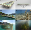 |
Fig. 2 Description of FLOLIZ. (A) & (B) − 3D side and profile design. Letters with a suffix number locate the different parts of the FLOLIZ detailed in each following panel; (A1) Floating part with helophytes; (A2) Underwater view of lateral part with empty wire cages; (B1) Juvenile Pike in 0.5 m-deep vegetation; (B2) Underwater view of 1m deep level with Potamogeton plant bed. ©UROS project (OFB-INRAE-ECOCEAN). |
2.3 Sampling stations
Three FLOLIZ were installed in downstream bays of the reservoir in September 2018 (Fig. 1B). The selected bays met the following criteria: a depth greater than 30 m to avoid the beaching of structures in winter when the water level is lowest, a low exposure to dominant winds to limit wave action, and an area of limited recreational activities. FLOLIZ area (70 m2) and depth (1 m maximum) was used to define the size of control stations located in the natural littoral zone (70 m long × 1 m wide and 1 m depth). Two types of control stations were chosen: one at the head of the bays in which FLOLIZ were installed (called NCS for Nearby Control Station) and another at the head of neighbouring bays in the same zone (called DCS for Distant Control Station) (Fig 1C). FLOLIZ could potentially have an influence over a certain area including the NCS; the comparison to DCS, considered far enough from FLOLIZ to be out of this influence radius, could then help to detect potential interactions between FLOLIZ and NCS. Each DCS was selected to be hydromorphologically similar to the NCS and located in the same zone (see Salmon et al., 2022).
2.4 Fish sampling
Fish were sampled in FLOLIZ and control stations in spring and summer from 2019 to 2022 using two non-lethal methods. Fish traps were used at night and visual census performed during daytime to get a complete picture of the fish community accounting for the diversity of daily activity patterns of species (Järvalt et al., 2005; Shoup et al., 2014). Spring and summer correspond to the peak activity period of fish and also give a good picture of the juvenile fish community (Fischer and Quist, 2014). In each season, the two sampling methods were carried out from one to four times (Table A1 in Appendix).
At night, eight unbaited fish traps (45 × 25 × 25 cm, mesh size 4 mm with an opening of 5 cm) were installed in FLOLIZ and control stations (DCS, NCS). In FLOLIZ, four fish traps were randomly placed in the 1 m deep underwater level and two fish traps in each 0.5 m deep underwater level (Fig. 3A). In control stations, fish traps were randomly placed in a 70-m2 area in the littoral zone. Similarly, in the underwater levels of FLOLIZ, four fish traps were placed at 0.5 m depth and four at 1 m depth in DCS and NCS (Fig. 3A). Fish traps were installed around 6 pm for an approximative duration of 15 h that included a few hours of daylight until dusk and a few hours of daylight after dawn. The next morning, the fish traps were removed and each fish was identified by species and measured (total length). A total of 1272 fish traps were collected (Table A1 in Appendix).
Visual census (snorkelling) was performed during daytime (Turner and Mackay, 1985; Brosse et al., 2001; Plichard et al., 2017). The high water transparency (4.5 m on average) made it possible to count fish and identify their species. Two qualified divers swam along each half of the 70 m-long linear transect in DCS and NCS and recorded all fish seen in the 1 m-wide band from the shoreline (Fig. 3B). The swimming speed was approximately 2 m min−1. The two divers took a census of FLOLIZ by first swimming around the structures and then inside them (Fig. 3B). During visual census, fish abundance was estimated based on a geometric progression factor: 1, 2–5, 6–10, 11–30, 31–50, 51–100, 101–200, 201–500, 500–1000 individuals (Harmelin-Vivien et al., 1985). The total length of individuals was estimated by using size markers. A total of 126 visual censuses were carried out (Table A1 in Appendix).
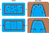 |
Fig. 3 Schematic drawing of the sampling protocols in FLOLIZ and control stations. (A) Fish trap sampling (during night) in FLOLIZ. Black squares symbolize fish traps; (B) Fish trap sampling in NCS and DCS. The white line marks the 0.5 m-deep littoral zone, the red one corresponds to the 1 m-deep one; (C) Visual census (daytime) in FLOLIZ. The dashed grey line with arrow symbolizes the swimming track of each diver; (D) Visual census (daytime) in NCS and DCS. |
2.5 Statistical analysis
To focus on the functionality of FLOLIZ, analyses have been carried out by separating juvenile and adult fish. The life stage was approximated by the total length. The classification was based on field data and literature data on the growth and maturity of the different species present in the Serre-Ponçon reservoir or in similar environments (Tab. A2 in Appendix). For each date and station, juvenile and adult fish abundance and species richness were calculated. For visual censuses, the total abundance was estimated by the center of the abundance classes (Harmelin-Vivien et al., 1985). Generalized linear models (GLM) were used to explain variations of abundance and species richness according to station type (FLOLIZ, DCS, NCS), season (Spring, Summer), year (2019, 2020, 2021, 2022) and their interactions (Zuur et al., 2009). For fish abundance, a negative binomial link function (Hardin & Hilbe 2007) was used to take into account over-dispersion and abundant zero values (Lindén and Mäntyniemi, 2011). For species richness, a Conway-Maxwell-Poisson link function, commonly used for count data, was used to take into account data that exhibit over- or under-dispersion (Sellers and Premeaux, 2021). GLM were performed with the “glmmTMB” R package (Brooks et al., 2017). The goodness of fit of each model was tested by using the ≪simulateResiduals≫ function in the “DHARMa” package which provided several plots and test functions to check for over/under-dispersion, zero inflation and spatial and temporal autocorrelation of residuals (Hartig and Lohse, 2022). A deviance analysis was run with the “Anova” function of the “car” package (Fox et al., 2001). For each significant effect, pairwise comparisons using marginal means estimated with a Tukey adjustment were carried out (“Emmeans” package ; Lenth, 2017).
To assess the composition of juvenile and adult fish communities and variations between station types over the whole sampling period, a non-metric multidimensional scaling (NMDS) ordination of fish species abundance was performed using the function ‘metaMDS’ in the vegan R package (Oksanen et al., 2001). Only species with a total abundance greater than 5 were selected. Species abundance was averaged by season for each year, to give each season the same weight in a year. These abundances were transformed into frequencies to get a species composition of 100% in each season of a year. The Bray-Curtis dissimilarity index was used to build a matrix of species frequencies among stations (Bray and Curtis, 1957). The goodness of fit of the NMDS was estimated with a stress function whose value inferior to 0.1 is great, to 0.2 is good, and to 0.3 corresponds to poor representation (Clarke, 1993). In addition, species abundance was compared between station type by using the Conover-Iman test (“Conover.test package” ; Dinno, 2015) with Holm p-value adjustment (Holm, 1979) which performs multiple comparisons using rank sums (Iman and Conover, 1979; Conover and Conover, 1999).
All statistical analyses were performed using R software version 4.4.1 (R Core Team, 2024) and RStudio software version 2022.12.0 (RStudio Team, 2022).
3 Results
3.1 Fish abundance and diversity
At night, a total of 938 juvenile and 172 adult fish from 10 species were captured by fish traps: 241 juvenile and 19 adults from 7 species in FLOLIZ, 330 juvenile and 101 adults from 9 species in DCS and 367 juvenile and 52 adults from 10 species in NCS.
At night, juvenile fish abundance differed between Season (P-value = 0.002), Year (P-value = 0.031), between Station according to Season (P-value = 0.043) and also according to Year (P-value = 0.007) (Tab. 1A). In the year 2019, mean juvenile abundance was higher in DCS and NCS than in FLOLIZ (Fig. 4A). In spring, in DCS (6.10 ± 15.3; P-value = 0.015) and NCS (5.62 ± 9.54; P-value = 0.020), mean juvenile abundance was higher than in FLOLIZ (1.28 ± 4.62) (Fig 4B). Juvenile species richness differed between Station, Year (P-value < 0.001 and < 0.001, respectively) and Season (P-value = 0.042) (Tab. 1A). More species were caught in DCS and NCS than in FLOLIZ (Fig. 4C). Adult fish abundance differed between Station (P-value = 0.009) and Year (P-value < 0.001) and adult species richness only differed between Year (P-value < 0.001). Finally, mean adult abundance was higher in DCS and NCS than in FLOLIZ (Fig. 4D).
During daytime, a total abundance of 4820 juveniles and 2119 adults fish from 12 species was estimated by visual census: 1297 juveniles and 1227 adults from 8 species in FLOLIZ; 1873 juveniles and 548 adults from 11 species in DCS; 1650 juveniles and 344 adults from 8 species in NCS. Juvenile fish species richness varied significantly between Season (P-value = 0.011) and between Station according to Year (P-value = 0.026). The species richness of juvenile fish was higher in DCS and NCS than in FLOLIZ in 2019 (Fig. 4E). Estimated abundance of juvenile fish differed only between Season (P-value = 0.002) (Tab. 2). For adult fish, estimated abundance differed significantly between Season (P-value = 0.002), between Year (P-value = 0.008) and between Station according to Year (P-value < 0.001). Adult fish were less abundant in FLOLIZ in 2019 than in NCS (Fig. 4F). They were more abundant in FLOLIZ than in littoral control stations in 2021 and more abundant than in DCS in 2022 (Fig. 4F). Adult species richness only differed between Season (P-value < 0.001).
Deviance analysis (ANOVA) for generalised linear models on fish abundance (Negative Binomial link function) and species richness (Conway-Maxwell-Poisson link function). (A) For juvenile and adult stage for fish trap sampling (night) and (B) For juvenile and adult stage for visual census sampling (daytime). Chisq = Wald Chisquare/Df = Deegre of freedom/Signification codes: *** for P-value < 0.001; ** for P-value < 0.01; * for P-value < 0.05.
 |
Fig. 4 Comparison of fish abundance and species richness at night (fish trap) and daytime (visual census). Only significant effects from the deviance analysis in Table 1 and ones that involve the type of station have been detailed to focus on the station effect. (A) Mean juvenile fish abundance (+ SD) between the different type of stations (DCS, NCS, FLOLIZ) according to year; (B) Mean juvenile fish abundance (+ SD) between the different type of stations (DCS, NCS, FLOLIZ) according to season; (C) Mean juvenile fish richness (+ SD) between the different type of stations; (D) Mean adult fish abundance (+ SD) between the different type of stations; (E) Mean adult fish richness (+ SD) between the different type of stations (DCS, NCS, FLOLIZ) according to year; (F) Mean adult fish abundance (+ SD) between the different type of stations (DCS, NCS, FLOLIZ) according to year. |
Mean frequencies ± SD of fish species in FLOLIZ and control stations (DCS, NCS) and pairwise comparisons with a Conover-Iman test between station type for night (A) and daytime (B) sampling over the whole sampling period (2019–2022). (NS = No significant/*** for P-value < 0.001/ ** for P-value < 0.01/ * for P-value < 0.05).
3.2 Fish community
The composition of fish communities appeared to be slightly different between FLOLIZ and control stations (Figs. 5A and 5B). At night, juvenile gudgeon, chub, perch and also adult blenny were more frequent in littoral communities than in FLOLIZ. During the day, FLOLIZ hosted a higher frequency of juvenile toxostoma (Chondrostoma toxostoma) and adult perch (Perca fluviatilis) compared to littoral communities. Juvenile gudgeon were also more frequent at daytime in DCS than in FLOLIZ. All the results are shown in Table 2.
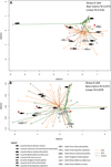 |
Fig. 5 Non-Metric Multidimensional Scaling ordination of fish species frequencies for FLOLIZ, NCS and DCS over the whole sampling period (2019–2022) at night (A) and during daytime (B). The stress value <0.20 corresponds to a good fit (Clarke, 1993). The non-metric fit R2 of 0.98 for both and the linear fit R2 of 0.92 and 0.88 respectively corresponds to a fairly good adjustment. The red stars (*) show a significant difference in the abundance of the corresponding species between the control stations (DCS, NCS) and the FLOLIZ (refer to Tab. 2). |
4 Discussion
Our results showed that abundance and species richness of fish at juvenile and adult stage in FLOLIZ could differ from those of littoral zones at different timescales, and, importantly, that this could coincide with differences in species assemblage.
4.1 Night use of FLOLIZ
At night, the littoral zone of the reservoir hosted greater fish abundance than FLOLIZ, particularly for juvenile gudgeon, perch, chub, and adult blenny, and higher richness. Gudgeon and blenny are two benthic fish species that preferred the fine substrates of debris cones in littoral zone at the head of the bay (Zweimuller, 1995; Mastrorillo et al., 1996; Gasith and Goren, 2009) rather than the coarse caged substrates of FLOLIZ. The swimming performance of benthic fish like gudgeon do not allow them to swim long distances in open water to reach the FLOLIZ (Tudorache et al., 2008). In addition, the riverine origin of gudgeon, chub, and blenny could explain their greater presence in littoral zones compared to FLOLIZ, which mimic small ponds where the flow to which these species are well adapted is dampened (Aarts et al., 2004; Wolter, 2010; Laporte et al., 2016). Finally, many studies have shown that juvenile perch increase their swimming activity at dusk and migrate in the littoral zone to forage and avoid predators in deep water (e.g. Wang and Eckmann, 1994; Jacobsen et al., 2015). At night, they rest on the bottom in the littoral zone (Imbrock et al., 1996).
4.2 Daytime use of FLOLIZ
During the day, differences of abundance between FLOLIZ and littoral zone could be observed from 2021. We could expect that the structured habitat within FLOLIZ attract fish during the daytime (Lewin et al., 2004; Maciej Gliwicz et al., 2006). In some years, abundance of fish in FLOLIZ could be higher than in littoral zones, FLOLIZ communities globally harboring more juvenile toxostoma and adult perch compared to that littoral areas that hosted more juvenile gudgeon. These results could strengthen the attractiveness of FLOLIZ due to the diversity and complexity of habitats they provide. In particular, aquatic vegetation increases the structural complexity and influences the distribution of fish (Thomaz and Cunha, 2010; Okun and Mehner, 2005). The early life stages of fish represent a critical period in their life cycle, due to high natural mortality and predation (Sifa and Mathias, 1987). The juvenile of toxostoma could take refuge in dense aquatic vegetation and in empty wire mesh cages of FLOLIZ to decrease predation risk (Persson and Eklov, 1995; Bry, 1996; Chick and Mlvor, 1997; Abdel-tawwab, 2005). Additionally, aquatic vegetation and complex structures support high food densities for fish (e.g. biofilm, plankton, macroinvertebrates) (Cazzanelli et al., 2008; Cremona et al., 2008; Jaschinski et al., 2011). This is suitable for toxostoma, which feed upon plankton, perilithon, and macroinvertebrates (Corse et al., 2010). By providing shelter and food, the aquatic vegetation appears to be an essential feature of habitats to support the survival and recruitment of many fish species (Rozas and Odum, 1988; Massicotte et al., 2015). Perch is a very plastic meso-predator which has been stocked since the Serre-Ponçon reservoir was built (Chappaz et al., 1998). The use of FLOLIZ by perch as a feeding ground results from the availability of prey, such as juvenile fish (mainly cyprinids) and the high abundance of macroinvertebrates (Salmon et al., 2022). Indeed, even at the adult stage, the perch diet is very generalist (Dörner et al., 2003). Moreover, the vegetation could provide a suitable spawning habitat for perch (Smith et al., 2001; Čech et al., 2009).
4.3 Attractiveness of FLOLIZ
Shortly after being installed, FLOLIZ became as attractive as littoral zones, at least during daytime. At night, FLOLIZ remained generally less attractive than littoral zones. These results differ significantly from other studies, which found an early and much higher use of AFI (Gillet, 1989; Nakamura et al., 1997; Huang et al., 2017; De Moraes et al., 2023) and other types of artificial structures (Santos et al., 2008, 2011; Feger and Spier, 2010). For example, Nakamura et al. (1997) found one hundred times more fish in AFI than in control areas in Lake Kasumigaura, Japan and De Moraes et al. (2023) observed densities of fish one to two order of magnitude greater in AFI than in their surroundings in Lipno Reservoir, Czech Republic. All these studies however show variable results with respect to the distribution of fish size; while De Moraes et al. (2023) and Santos et al. (2008) found more small fish in AFI, Huang et al. (2017) and Feger et al. (2010) did not. Some design differences with our study are worth emphasizing. Nakamura et al. (1997) tested a much bigger structure (the size of their AFI was 874 m2) than ours (70 m2), which could have played a role, for example, given the space requirements for pike spawning grounds and home ranges (Chancerel, 2003; Cook and Bergersen, 1988; Sandlund et al., 2016). De Moraes et al. (2023) used smaller structures (10 or 14 m2), but also a greater number of them distributed in closer proximity, and still observed higher fish densities. Another big difference with our study is the littoral location of artificial structures. In De Moraes et al. (2023), structures were located in water at a depth of 1.5 to 1.7 m and very close to the shore; structures were also situated close to the shore in Nakamura et al. (1997). This is also the case for artificial reefs, which are often located in the shallow littoral zone (Kelch et al., 1999; Schou et al., 2009; Feger and Spier, 2010; Baumann et al., 2016). This location in the natural littoral area contrasts with our FLOLIZ, which are located about 50 m offshore in waters as deep as 30 m due to constraints linked to extremely high annual WLF (Salmon et al., 2022). This disconnection from the littoral area could have limited the colonization of FLOLIZ; small individuals and benthic species with reduced swimming performance (Ojanguren and Braña, 2003; Tudorache et al., 2008) could fear to swim across a risky pelagic area to reach FLOLIZ (Braband and Faafeng, 1993; Shoup et al., 2014). Gillet (1989) however observed various species such as perch, pike and cyprinids spawning on artificial grounds that could be far from the bank in lakeshore zones of large lakes but without any evaluation of fish densities. The relatively small area of offshore FLOLIZ could be difficult for fish to find and could therefore be a limiting factor in their efficiency. Differences in physico-chemical factors, which have an effect on the attractiveness of artificial structures (Walters et al., 1991; Moring and Nicholson, 1994), could also be involved. Indeed, in these studies showing a positive effect of AFIs on fish, AFIs were installed in sites very different from Serre-Ponçon: much shallower (∼5 m), with much lower WLF (up to 3 m), and with eutrophic water.
Studies testing structures comparable to FLOLIZ aiming at providing both spawning substrates and nursery habitats remain scarce and further research into the effectiveness of FLOLIZ in different environmental contexts or with different designs is needed and could offer mitigation solutions against the deleterious effects of WLF, at least for some targeted species. For example, juvenile northern pike seemed to be characteristic of the FLOLIZ community with more frequent observations than in littoral stations during daytime but with a high variability between sampling campaigns. A focus on this species with a slightly different analysis and time period led to some positive effect of FLOLIZ on pike abundance, even if weak (Salmon et al., 2024). This suggests that there may be a positive signal for some species. In Serre-Ponçon reservoir, other phytophilous species are present (i.e. tench, carp) but they are less frequent in its downstream section characterized by steep and homogeneous banks and great depths. Studies have shown that there is an upstream/downstream gradient in fish abundance and biomass in reservoirs (Anderson et al., 1983; Swierzowski, 2000; Prchalová et al., 2008, 2009) due to differences in productivity and littoral habitats. Therefore, it would be interesting to implement new FLOLIZ in the upstream part of the reservoir in order to assess their attractiveness for other species.
Finally, we find it useful to mention that no crayfish were caught or seen in FLOLIZ over these four years even though an exotic species (Faxonius limosus) is present in Serre-Ponçon. The disconnection of FLOLIZ from the bank and from the bottom very probably prevented their colonization by crayfish; amphibians (Bufo bufo) and their eggs, however, were seen in FLOLIZ.
4.4 Methodological considerations
The use of two different methods with fish traps at night and visual census during daytime did not allow for comparisons between night and day but did allow for the comparison of FLOLIZ with control stations. With passive capture, traps sampled the most mobile fish whereas visual census sampled both mobile and less mobile ones; but visual census probably underestimated the number of individuals in FLOLIZ compared to the littoral zone as fish can hide in numerous cavities, dense vegetation or be hidden by the FLOLIZ structures. Finally, the size of the trap was a limiting factor for the capture of large adult individuals. However, taking into consideration the species sampled during this study, only adult pike and large chub could not be captured by the fish traps.
5 Conclusion
The lack of littoral habitats, and particularly refuge and nursery habitats for juvenile fish, can lead to a decline in some populations in reservoirs subject to WLF. By mimicking the habitats of a littoral zone, FLOLIZ could be a potential mitigation solution for such lake ecosystems. This study showed that abundance and richness of both adult and juvenile fish were comparable between FLOLIZ and littoral stations during the day, while at night fish were more abundant in littoral stations, even if this is not generalized to all species. These results show that fish can indeed use FLOLIZ but probably not in a way that could mitigate the deleterious effects of WLF on fish populations. Such studies remain scarce and further ones should be encouraged in other reservoirs (with different sizes and amplitudes of WLF) or other types of artificial lakes (for example, hill reservoirs) and with different FLOLIZ designs in order to obtain robust conclusions on their potential effectiveness.
Acknowledgements
The French Biodiversity Agency (OFB), the French National Research Institute for Agriculture, Food and Environment (INRAE), the ECOCEAN Company and the French National Agency for Research and Technology (ANRT) performed this research and development study. We are grateful to the stakeholders of Serre-Ponçon reservoir (S.M.A.D.E.S.E.P.: Syndicat Mixte d’Aménagement et de Développement du Lac de Serre-Ponçon) for their enthusiastic support and their assistance in setting up the FLOLIZ. We would like to thank all the local organisations for hosting the project, their contributions and their interest in its development (Comission de Serre-Ponçon, CBNA “Conservatoire Botanique National Alpin”, EDF “Electricité de France”, Fishing federation of Hautes-Alpes and Alpes-de-Haute-Provence, DDT “Direction Départementale des Territoires des Hautes-Alpes et des Alpes-de-Haute-Provence). We would like to thank all those who provided field assistance (i.e. Tiphaine PEROUX, Dorian MILESI, Nathalie REYNAUD, the OFB 05 departmental service team). Thank to Remy DUBAS (ECOCEAN) for the high-quality pictures of the FLOLIZ. We thank EDF for sharing water level data and an anonymous reviewer and the editor-in-chief of the journal for their valuable comments that helped to improve the paper.
Supplementary Material
Figure A1. Daily variations of the elevation of Serre-Ponçon reservoir between 2017 and 2022 (Data from EDF).
Figure A2. Fitness of generalised linear models (GLM) by DHARMa package. A – Juvenile abundance for visual census sampling; B – Juvenile species richness for visual census sampling; C – Juvenile abundance for fish trap sampling; D – Juvenile species richness for fish trap sampling; E – Adult abundance for visual census sampling; F – Adult species richness for visual census sampling; G – Adult abundance for fish trap sampling; H – Adult species richness for fish trap sampling.
Table A1. Overview of samplings carried out by method and season year.
Table A2. Summary of estimated maturity size (total length) for different fishes in Serre-Ponçon reservoir or in similar environments based on literature.
Access Supplementary MaterialReferences
- Aarts BGW, Van Den Brink FWB, Nienhuis PH. 2004. Habitat loss as the main cause of the slow recovery of fish faunas of regulated large rivers in Europe: the transversal floodplain gradient. River Res Appl 20: 3–23. [CrossRef] [Google Scholar]
- Abdel-tawwab M. 2005. The effect of artificial vegetation density on growth and growth related parameters of Nile Tilapia, Oreochromis niloticus (L.) Fry. Turk J Fish Aquat Sci 5: 63–68. [Google Scholar]
- Anderson KA, Beitinger TL, Zimmerman EG. 1983. Forage fish assemblages in the Brazos river upstream and downstream from Possum Kingdom Reservoir, Texas. J Freshw Ecol 2: 81–88. [CrossRef] [Google Scholar]
- Baumann JR, Oakley NC, McRae BJ. 2016. Evaluating the effectiveness of artificial fish habitat designs in turbid reservoirs using sonar imagery. North Am J Fish Manag 36: 1437–1444. [CrossRef] [Google Scholar]
- Brabrand Å, Faafeng B. 1993. Habitat shift in roach (Rutilus rutilus) induced by pikeperch (Stizostedion lucioperca) introduction: predation risk versus pelagic behaviour. Oecologia 95: 38–46. [CrossRef] [PubMed] [Google Scholar]
- Bray JR, Curtis JT. 1957. An ordination of the upland forest communities of Southern Wisconsin. Ecol Monogr 27: 326–349. [Google Scholar]
- Brooks ME, Kristensen K, Benthem KJ, van, Magnusson A, Berg CW, Nielsen A, Skaug HJ, Mächler M, Bolker BM. 2017. glmmTMB balances speed and flexibility among packages for zero-inflated generalized linear mixed modeling. R J 9: 378. [CrossRef] [Google Scholar]
- Brosse S, Laffaille P, Gabas S, Lek S. 2001. Is scuba sampling a relevant method to study fish microhabitat in lakes? Examples and comparisons for three European species. Ecol Freshw Fish 10: 138–146. [CrossRef] [Google Scholar]
- Bry C. 1996. Role of vegetation in the life cycle of pike. Pike: biology and exploitation. Springer, pp. 45–67. [Google Scholar]
- Carmignani JR, Roy AH, Hazelton PD, Giard H. 2019. Annual winter water level drawdowns limit shallow-water mussel densities in small lakes. Freshw Biol 64: 1519–1533. [CrossRef] [Google Scholar]
- Cazzanelli M, Warming TP, Christoffersen KS. 2008. Emergent and floating-leaved macrophytes as refuge for zooplankton in a eutrophic temperate lake without submerged vegetation. Hydrobiologia 605: 113–122. [CrossRef] [Google Scholar]
- Čech M, Peterka J, Říha M, Jůza T, Kubečka J. 2009. Distribution of egg strands of perch (Perca fluviatilis L.) with respect to depth and spawning substrate. Hydrobiologia 630: 105–114. [CrossRef] [Google Scholar]
- Chancerel F. 2003. Le brochet, Biologie et gestion. CSP Ed., Collection Mise au point. [Google Scholar]
- Chappaz R, Doucende D, Barthelemy R. 1998. Patterns of change in zooplankton community structures and the selective feeding of Bleak, Alburnus alburnus (L.) in the Serre Ponçon dam between 1980 and 1996. [Google Scholar]
- Chick JH, Mlvor CC. 1997. Habitat selection by three littoral zone fishes: effects of predation pressure, plant density and macrophyte type. Ecol Freshw Fish 6: 27–35. [CrossRef] [Google Scholar]
- Clarke KR. 1993. Non-parametric multivariate analyses of changes in community structure. Aust J Ecol 18: 117–143. [CrossRef] [Google Scholar]
- Conover WJ, Conover WJ. 1999. Practical nonparametric statistics. New York, NY/Weinheim: Wiley, 584p. [Google Scholar]
- Cook MF, Bergersen EP. 1988. Movements, habitat selection, and activity periods of northern pike in Eleven Mile Reservoir, Colorado. Trans Am Fish Soc 117: 495–502. [CrossRef] [Google Scholar]
- Coops H, Beklioglu M, Crisman TL. 2003. The role of water-level fluctuations in shallow lake ecosystems − workshop conclusions. Hydrobiologia 506–509: 23–27. [CrossRef] [Google Scholar]
- Corse E, Costedoat C, Chappaz R, Pech N, Martin J-F, Gilles A. 2010. A PCR-based method for diet analysis in freshwater organisms using 18S rDNA barcoding on faeces. Mol Ecol Resour 10: 96–108. [CrossRef] [PubMed] [Google Scholar]
- Cremona F, Planas D, Lucotte M. 2008. Biomass and composition of macroinvertebrate communities associated with different types of macrophyte architectures and habitats in a large fluvial lake. Fundam Appl Limnol 171: 119–130. [CrossRef] [Google Scholar]
- Czarnecka M. 2016. Coarse woody debris in temperate littoral zones: implications for biodiversity, food webs and lake management. Hydrobiologia 767: 13–25. [CrossRef] [Google Scholar]
- De Moraes KR, Souza AT, Muška M, Hladík M, Čtvrtlíková M, Draštík V, Kolařík T, Kučerová A, Krolová M, Sajdlová Z, Šmejkal M, Kubečka J. 2023. Artificial floating islands: a promising tool to support juvenile fish in lacustrine systems. Hydrobiologia 850: 1969–1984. [CrossRef] [Google Scholar]
- Dinno A. 2015. conover.test: Conover-Iman Test of Multiple Comparisons Using Rank Sums. 1.1.6. [Google Scholar]
- Dörner H, Berg S, Jacobsen L, Hülsmann S, Brojerg M, Wagner A. 2003. The feeding behaviour of large perch Perca fluviatilis (L.) in relation to food availability: a comparative study. Hydrobiologia 506–509: 427–434. [CrossRef] [Google Scholar]
- Evtimova VV, Donohue I. 2016. Water-level fluctuations regulate the structure and functioning of natural lakes. Freshw Biol 61: 251–264. [CrossRef] [Google Scholar]
- Farrell JM. Reproductive Success of Sympatric Northern Pike and Muskellunge in an Upper St. Lawrence River Bay. [Google Scholar]
- Feger BT, Spier TW. 2010. Evaluation of artificial PVC pipe structures as fish habitat in Spring Lake, Western Illinois, USA. Lakes Reserv Sci Policy Manag Sustain Use 15: 335–340. [Google Scholar]
- Fischer JR, Quist MC. 2014. Gear and seasonal bias associated with abundance and size structure estimates for lentic freshwater fishes. J Fish Wildl Manag 5: 394–412. [CrossRef] [Google Scholar]
- Fischer P, Öhl U. 2005. Effects of water-level fluctuations on the littoral benthic fish community in lakes: a mesocosm experiment. Behav Ecol 16: 741–746. [CrossRef] [Google Scholar]
- Fox J, Weisberg S, Price B. 2001. car: Companion to Applied Regression. 3: 1–2. [Google Scholar]
- Furey PC, Nordin RN, Mazumder A. 2004. Water level drawdown affects physical and biogeochemical properties of littoral sediments of a reservoir and a natural lake. Lake Reserv Manag 20: 280–295. [CrossRef] [Google Scholar]
- Gasith A, Goren M. 2009. Habitat availability, reproduction and population dynamics of the fresh water blenny Salaria fluviatilis (asso, 1801) in Lake Kinneret, Israel. Electron J Ichthyol 2: 34–46. [Google Scholar]
- Gillet C. 1989. Réalisation de frayères artificielles flottantes pour les poissons lacustres. Hydroécolog Appl 1: 145–193. [CrossRef] [EDP Sciences] [Google Scholar]
- Grabowski TB, Isely JJ. 2007. Effects of flow fluctuations on the spawning habitat of a riverine fish. Southeast Nat 6: 471–478. [CrossRef] [Google Scholar]
- Harmelin-Vivien ML, Harmelin JG, Chauvet C, Mellon-Duval C, Galzin R, Lejeune P, Barnabé G, Blanc F, Chevalier R, Duclerc J, Lasserre G. 1985. Evaluation visuelle des peuplements et populations de poissons: méthodes et problèmes. Rev DÉcologie Terre Vie 40: 467–539. [CrossRef] [Google Scholar]
- Hartig F, Lohse L. 2022. DHARMa: Residual Diagnostics for Hierarchical (Multi-Level / Mixed) Regression Models. [Google Scholar]
- Haxton TJ, Findlay CS. 2009. Variation in large-bodied fish-community structure and abundance in relation to water-management regime in a large regulated river. J Fish Biol 74: 2216–2238. [CrossRef] [PubMed] [Google Scholar]
- Hirsch PE, Schillinger S, Weigt H, Burkhardt-Holm P. 2014. A hydro-economic model for water level fluctuations: combining limnology with economics for sustainable development of hydropower. Pandit MK, ed. PLoS ONE 9: e114889. [CrossRef] [PubMed] [Google Scholar]
- Holm S. 1979. A simple sequentially rejective multiple test procedure. Scand J Stat 6: 65–70. [Google Scholar]
- Huang X, Zhao F, Song C, Gao Y, Geng Z, Zhuang P. 2017. Effects of stereoscopic artificial floating wetlands on nekton abundance and biomass in the Yangtze Estuary. Chemosphere 183: 510–518. [CrossRef] [PubMed] [Google Scholar]
- Iman RL, Conover WJ. 1979. The use of the rank transform in regression. Technometrics 21: 499–509. [CrossRef] [Google Scholar]
- Imbrock F, Appenzeller A, Eckmann R. 1996. Diel and seasonal distribution of perch in Lake Constance: a hydroacoustic study and in situ observations. J Fish Biol 49: 1–13. [Google Scholar]
- Jacobsen L, Berg S, Baktoft H, Skov C. 2015. Behavioural strategy of large perch Perca fluviatilis varies between a mesotrophic and a hypereutrophic lake. J Fish Biol 86: 1016–1029. [CrossRef] [PubMed] [Google Scholar]
- Järvalt A, Krause T, Palm A. 2005. Diel migration and spatial distribution of fish in a small stratified lake. In Ott I, Kõiv T, eds. Lake Verevi, Estonia — A Highly Stratified Hypertrophic Lake, Springer Netherlands, Dordrecht. 197–203. [Google Scholar]
- Jaschinski S, Brepohl DC, Sommer U. 2011. The trophic importance of epiphytic algae in a freshwater macrophyte system (Potamogeton perfoliatus L.): stable isotope and fatty acid analyses. Aquat Sci 73: 91–101. [CrossRef] [Google Scholar]
- Kahl U, Hülsmann S, Radke RJ, Benndorf J. 2008. The impact of water level fluctuations on the year class strength of roach: implications for fish stock management. Limnologica 38: 258–268. [CrossRef] [Google Scholar]
- Kelch DO, Snyder FL, Reutter JM. 1999. Artificial Reefs in Lake Erie: Biological Impacts of Habitat Alteration. In : Am. Fish. Soc. Symp. 1999: 335–347. [Google Scholar]
- Laporte M, Claude J, Berrebi P, Perret P, Magnan P. 2016. Shape plasticity in response to water velocity in the freshwater blenny Salaria fluviatilis. J Fish Biol 88: 1191–1203. [CrossRef] [PubMed] [Google Scholar]
- Leira M, Cantonati M. 2008. Effects of water-level fluctuations on lakes: an annotated bibliography. In Wantzen KM, Rothhaupt K-O, Mörtl M, Cantonati M, −Tóth LG, Fischer P, eds. Ecological Effects of Water-Level Fluctuations in Lakes. Netherlands, Dordrecht: Springer, pp. 171–184. [Google Scholar]
- Lenth RV. 2017. emmeans: Estimated Marginal Means, aka Least-Squares Means. 1.10.3. [Google Scholar]
- Lewin W-C, Okun N, Mehner T. 2004. Determinants of the distribution of juvenile fish in the littoral area of a shallow lake. Freshw Biol 49: 410–424. [CrossRef] [Google Scholar]
- Lindén A, Mäntyniemi S. 2011. Using the negative binomial distribution to model overdispersion in ecological count data. Ecology 92: 1414–1421. [CrossRef] [PubMed] [Google Scholar]
- Logez M, Roy R, Tissot L, Argillier C. 2016. Effects of water-level fluctuations on the environmental characteristics and fish-environment relationships in the littoral zone of a reservoir. Fundam Appl Limnol 189: 37–49. [CrossRef] [Google Scholar]
- Maciej Gliwicz Z, Slon J, Szynkarczyk I. 2006. Trading safety for food: evidence from gut contents in roach and bleak captured at different distances offshore from their daytime littoral refuge. Freshw Biol 51: 823–839. [CrossRef] [Google Scholar]
- Maday A, Matern S, Monk CT, Klefoth T, Wolter C, Arlinghaus R. 2023. Seasonal and diurnal patterns of littoral microhabitat use by fish in gravel pit lakes, with special reference to supplemented deadwood brush piles. Hydrobiologia 850: 1557–1581. [CrossRef] [Google Scholar]
- Massicotte P, Bertolo A, Brodeur P, Hudon C, Mingelbier M, Magnan P. 2015. Influence of the aquatic vegetation landscape on larval fish abundance. J Gt Lakes Res 41: 873–880. [CrossRef] [Google Scholar]
- Mastrorillo S, Dauba F, Belaud A. 1996. Utilisation des microhabitats par le vairon, le goujon et la loche franche dans trois rivières du sud-ouest de la France. Ann Limnol − Int J Limnol 32: 185–195. [CrossRef] [EDP Sciences] [Google Scholar]
- McDowell CP. 2012. Winter Drawdown Effects on Swim-up Date and Growth Rate of Age-0 Fishes in Connecticut. University of Connecticut. [Google Scholar]
- Meerhoff M, de los Ángeles González-Sagrario M. 2022. Habitat complexity in shallow lakes and ponds: importance, threats, and potential for restoration. Hydrobiologia 849: 3737–3760. [Google Scholar]
- Moring JR, Nicholson PH. 1994. Evaluation of Three Types of Artificial Habitats for Fishes in a Freshwater Pond in Maine, USA. [Google Scholar]
- Nakamura K, Tsukidate M, Shimatani Y. 1997. Characteristic of Ecosystem of an Artificial Vegetated Floating Island. WIT Transactions on Ecology and the Environment WIT Press 22. [Google Scholar]
- Nakamura K, Mueller G. 2008. Review of the Performance of the Artificial Floating Island as a Restoration Tool for Aquatic Environments. World Environmental and Water Resources Congress 2008, American Society of Civil Engineers, Honolulu, Hawaii, United States, 1–10. [Google Scholar]
- Ojanguren AF, Braña F. 2003. Effects of size and morphology on swimming performance in juvenile brown trout (Salmo trutta L.). Ecol Freshwater Fish 12: 241–246. [CrossRef] [Google Scholar]
- Oksanen J, Simpson GL, Blanchet FG, Kindt R, Legendre P, Minchin PR, O’Hara RB, Solymos P, Stevens MHH, Szoecs E, Wagner H, Barbour M, Bedward M, Bolker B, Borcard D, Carvalho G, Chirico M, De Caceres M, Durand S, Evangelista HBA, FitzJohn R, Friendly M, Furneaux B, Hannigan G, Hill MO, Lahti L, McGlinn D, Ouellette M-H, Ribeiro Cunha E, Smith T, Stier A, Ter Braak CJF, Weedon J. 2001. vegan: Community Ecology Package. 2.6–6.1. [Google Scholar]
- Okun N, Mehner T. 2005. Distribution and feeding of juvenile fish on invertebrates in littoral reed (Phragmites) stands. Ecol Freshw Fish 14: 139–149. [CrossRef] [Google Scholar]
- Pedicillo G, Merulli F, Carosi A, Viali P, Lorenzoni M. 2008. The use of artificial spawning substrates as media to support the reproduction of Eurasian perch in Lake Piediluco. Hydrobiologia 609: 219–223. [CrossRef] [Google Scholar]
- Persson L, Eklov P. 1995. Prey refuges affecting interactions between piscivorous Perch and Juvenile Perch and Roach. Ecology 76: 70–81. [CrossRef] [Google Scholar]
- Plichard L, Capra H, Mons R, Pella H, Lamouroux N. 2017. Comparing electrofishing and snorkelling for characterizing fish assemblages over time and space. Can J Fish Aquat Sci 74: 75–86. [CrossRef] [Google Scholar]
- Prashant, Billore SK. 2020. Macroinvertebrates associated with artificial floating islands installed in River Kshipra for water quality improvement. Water Sci Technol 81: 1242–1249. [CrossRef] [PubMed] [Google Scholar]
- Prchalová M, Kubečka J, Vašek M, Peterka J, Sed’a J, Jůza T, Říha M, Jarolím O, Tušer M, Kratochvíl M, ČEch M, Draštík V, Frouzová J, Hohausová E. 2008. Distribution patterns of fishes in a canyon-shaped reservoir. J Fish Biol 73: 54–78. [CrossRef] [Google Scholar]
- Prchalová M, Kubečka J, Čech M, Frouzová J, Draštík V, Hohausová E, Jůza T, Kratochvíl M, Matěna J, Peterka J, Říha M, Tušer M, Vašek M. 2009. The effect of depth, distance from dam and habitat on spatial distribution of fish in an artificial reservoir. Ecol Freshw Fish 18: 247–260. [CrossRef] [Google Scholar]
- Říha M, Kubečka J, Prchalová M, Mrkvička T, Čech M, Draštík V, Frouzová J, Hohausová E, Jůza T, Kratochvíl M, Peterka J, Tušer M, Vašek M. 2011. The influence of diel period on fish assemblage in the unstructured littoral of reservoirs. Fish Manag Ecol 18: 339–347. [CrossRef] [Google Scholar]
- Rozas LP, Odum WE. 1988. Occupation of submerged aquatic vegetation by fishes: testing the roles of food and refuge. Oecologia 77: 101–106. [CrossRef] [PubMed] [Google Scholar]
- Sala MM, Güde H. 2006. Seasonal dynamics of pelagic and benthic (littoral and profundal) bacterial abundances and activities in a deep prealpine lake (L. Constance). Arch Für Hydrobiol 167: 351–369. [CrossRef] [Google Scholar]
- Salmon Q, Colas F, Westrelin S, Dublon J, Baudoin J-M. 2022. Floating Littoral Zone (FLOLIZ): A solution to sustain macroinvertebrate communities in regulated lakes? Ecol Eng 176: 106509. [CrossRef] [Google Scholar]
- Salmon Q, Westrelin S, Dublon J, Abadie E, Baudoin J-M. 2024. Artificial floating littoral zones: a promising nursery to support Pike (Esox lucius) in reservoirs. Int J Limnol 60: 22. [CrossRef] [EDP Sciences] [Google Scholar]
- Sandlund OT, Museth J, Øistad S. 2016. Migration, growth patterns, and diet of pike (Esox lucius) in a river reservoir and its inflowing river. Fish Res 173: 53–60. [Google Scholar]
- Santos LN, Araújo FG, Brotto DS. 2008. Artificial structures as tools for fish habitat rehabilitation in a neotropical reservoir. Aquat Conserv Mar Freshw Ecosyst 18: 896–908. [CrossRef] [Google Scholar]
- Santos LN, García-Berthou E, Agostinho AA, Latini JD. 2011. Fish colonization of artificial reefs in a large Neotropical reservoir: material type and successional changes. Ecol Appl 21: 251–262. [CrossRef] [PubMed] [Google Scholar]
- Sellers KF, Premeaux B. 2021. Conway-Maxwell-Poisson regression models for dispersed count data. WIREs Comput Stat 13: e1533. [CrossRef] [Google Scholar]
- Schou MO, Risholt C, Lauridsen TL, Søndergaard M, Grønkjær P, Jacobsen L, Berg S, Skov C, Brucet S, Jeppesen E. 2009. Restoring lakes by using artificial plant beds habitat selection of zooplankton in a clear and a turbid shallow lake. Freshw Biol 54: 1520–1531. [CrossRef] [Google Scholar]
- Shoup DE, Boswell KM, Wahl DH. 2014. Diel Littoral-Pelagic Movements by Juvenile Bluegills in a small lake. Trans Am Fish Soc 143: 796–801. [CrossRef] [Google Scholar]
- Sifa L, Mathias JA. 1987. The critical period of high mortality of larvae fish—a discussion based on current research. Chin J Oceanol Limnol 5: 80–96. [CrossRef] [Google Scholar]
- Smith C, Douglas A, Jurajda P. 2001. Oviposition site selection and embryo mortality in perch. J Fish Biol 58: 880–882. [CrossRef] [Google Scholar]
- Sutela T, Vehanen T, Rask M. 2011. Assessment of the ecological status of regulated lakes: stressor-specific metrics from littoral fish assemblages. Hydrobiologia 675: 55–64. [CrossRef] [Google Scholar]
- Sutela T, Aroviita J, Keto A. 2013. Assessing ecological status of regulated lakes with littoral macrophyte, macroinvertebrate and fish assemblages. Ecol Indic 24: 185–192. [CrossRef] [Google Scholar]
- Swierzowski A. 2000. The relationship between the spatial distribution of fish, zooplankton and other environmental parameters in the Solina reservoir, Poland. Aquat Living Resour 13: 373–377. [CrossRef] [Google Scholar]
- Thomaz SM, Cunha ER da. 2010. The role of macrophytes in habitat structuring in aquatic ecosystems: methods of measurement, causes and consequences on animal assemblages’ composition and biodiversity. Acta Limnolog Brasiliensia 22: 218–236. [CrossRef] [Google Scholar]
- Trussart S, Messier D, Roquet V, Aki S. 2002. Hydropower projects: a review of most effective mitigation measures. Energy Policy 30: 1251–1259. [CrossRef] [Google Scholar]
- Tudorache C, Viaene P, Blust R, Vereecken H, De Boeck G. 2008. A comparison of swimming capacity and energy use in seven European freshwater fish species. Ecol Freshw Fish 17: 284–291. [CrossRef] [Google Scholar]
- Tundisi JG, Matsumura-Tundisi T. 2003. Integration of research and management in optimizing multiple uses of reservoirs: the experience in South America and Brazilian case studies. In: Martens K, ed. Aquatic Biodiversity: A Celebratory Volume in Honour of Henri J. Dumont. Netherlands, Dordrecht: Springer, pp. 231–242. [Google Scholar]
- Turner LJ, Mackay WC. 1985. Use of Visual Census for Estimating Population Size in Northern Pike (Esox lucius). https://cdnsciencepub.com/doi/abs/10.1139/f85-231 (accessed July 22, 2024). [Google Scholar]
- Walters DA, Lynch WE, Johnson DL. 1991. How depth and interstice size of artificial structures influence fish attraction. North Am J Fish Manag 11: 319–329. [CrossRef] [Google Scholar]
- Wang N, Eckmann R. 1994. Distribution of perch (Perca fluviatilis L.) during their first year of life in Lake Constance. Hydrobiologia 277: 135–143. [CrossRef] [Google Scholar]
- Westrelin S, Cucherousset J, Roy R, Tissot L, Santoul F, Argillier C. 2022. Habitat partitioning among three predatory fish in a temperate reservoir. Ecol Freshw Fish 31: 129–142. [CrossRef] [Google Scholar]
- Winfield IJ. 2004. Fish in the littoral zone: ecology, threats and management. Limnologica 34: 124–131. [CrossRef] [Google Scholar]
- Wolcox DA, Meeker JE. 1992. Implications for faunal habitat related to altered macrophyte structure in regulated lakes in northern Minnesota. Wetlands 12: 192–203. [CrossRef] [Google Scholar]
- Wolter C. 2010. Functional vs scenic restoration − challenges to improve fish and fisheries in urban waters. Fish Manag Ecol 17: 176–185. [CrossRef] [Google Scholar]
- Yeh N, Yeh P, Chang Y-H. 2015. Artificial floating islands for environmental improvement. Renew Sustain Energy Rev 47: 616–622. [CrossRef] [Google Scholar]
- Zohary T, Gasith A. 2014. The Littoral Zone. In Zohary T, Sukenik A, Berman T, Nishri A, eds. Lake Kinneret. Dordrecht: Springer Netherlands, pp. 517–532. [Google Scholar]
- Zuur AF, Ieno EN, Walker NJ, Saveliev AA, Smith GM. 2009. GLM and GAM for count data. In Zuur AF, Ieno EN, Walker N, Saveliev AA, Smith GM, eds. Mixed effects models and extensions in ecology with R. New York, NY: Springer, pp. 209–243. [Google Scholar]
- Zweimuller I. 1995. Microhabitat use by two small benthic stream fish in a 2nd order stream. Hydrobiologia 303: 125–137. [CrossRef] [Google Scholar]
Cite this article as: Salmon Q, Westrelin S, Dublon J, Fonbonne S, Baudoin J-M. 2025. An evaluation of artificial floating littoral zones to support fish communities in reservoirs. Knowl. Manag. Aquat. Ecosyst., 426, 3
All Tables
Deviance analysis (ANOVA) for generalised linear models on fish abundance (Negative Binomial link function) and species richness (Conway-Maxwell-Poisson link function). (A) For juvenile and adult stage for fish trap sampling (night) and (B) For juvenile and adult stage for visual census sampling (daytime). Chisq = Wald Chisquare/Df = Deegre of freedom/Signification codes: *** for P-value < 0.001; ** for P-value < 0.01; * for P-value < 0.05.
Mean frequencies ± SD of fish species in FLOLIZ and control stations (DCS, NCS) and pairwise comparisons with a Conover-Iman test between station type for night (A) and daytime (B) sampling over the whole sampling period (2019–2022). (NS = No significant/*** for P-value < 0.001/ ** for P-value < 0.01/ * for P-value < 0.05).
All Figures
|
Fig. 1 Location of FLOLIZ and control stations in Serre-Ponçon hydropower reservoir. (A) Location of Serre-Ponçon hydropower reservoir in France; (B) Reservoir contour at the highest water level (altitude 780 m) and location of 3 sampling zones (ellipses); (C) Focus on the 3 zones (suffixed 1, 2 and 3) with control stations and FLOLIZ. DCS: Distant Control Station, NCS: Nearby Control Station, FLOLIZ: Floating Littoral Zone. |
| In the text | |
|
Fig. 2 Description of FLOLIZ. (A) & (B) − 3D side and profile design. Letters with a suffix number locate the different parts of the FLOLIZ detailed in each following panel; (A1) Floating part with helophytes; (A2) Underwater view of lateral part with empty wire cages; (B1) Juvenile Pike in 0.5 m-deep vegetation; (B2) Underwater view of 1m deep level with Potamogeton plant bed. ©UROS project (OFB-INRAE-ECOCEAN). |
| In the text | |
|
Fig. 3 Schematic drawing of the sampling protocols in FLOLIZ and control stations. (A) Fish trap sampling (during night) in FLOLIZ. Black squares symbolize fish traps; (B) Fish trap sampling in NCS and DCS. The white line marks the 0.5 m-deep littoral zone, the red one corresponds to the 1 m-deep one; (C) Visual census (daytime) in FLOLIZ. The dashed grey line with arrow symbolizes the swimming track of each diver; (D) Visual census (daytime) in NCS and DCS. |
| In the text | |
|
Fig. 4 Comparison of fish abundance and species richness at night (fish trap) and daytime (visual census). Only significant effects from the deviance analysis in Table 1 and ones that involve the type of station have been detailed to focus on the station effect. (A) Mean juvenile fish abundance (+ SD) between the different type of stations (DCS, NCS, FLOLIZ) according to year; (B) Mean juvenile fish abundance (+ SD) between the different type of stations (DCS, NCS, FLOLIZ) according to season; (C) Mean juvenile fish richness (+ SD) between the different type of stations; (D) Mean adult fish abundance (+ SD) between the different type of stations; (E) Mean adult fish richness (+ SD) between the different type of stations (DCS, NCS, FLOLIZ) according to year; (F) Mean adult fish abundance (+ SD) between the different type of stations (DCS, NCS, FLOLIZ) according to year. |
| In the text | |
|
Fig. 5 Non-Metric Multidimensional Scaling ordination of fish species frequencies for FLOLIZ, NCS and DCS over the whole sampling period (2019–2022) at night (A) and during daytime (B). The stress value <0.20 corresponds to a good fit (Clarke, 1993). The non-metric fit R2 of 0.98 for both and the linear fit R2 of 0.92 and 0.88 respectively corresponds to a fairly good adjustment. The red stars (*) show a significant difference in the abundance of the corresponding species between the control stations (DCS, NCS) and the FLOLIZ (refer to Tab. 2). |
| In the text | |
Current usage metrics show cumulative count of Article Views (full-text article views including HTML views, PDF and ePub downloads, according to the available data) and Abstracts Views on Vision4Press platform.
Data correspond to usage on the plateform after 2015. The current usage metrics is available 48-96 hours after online publication and is updated daily on week days.
Initial download of the metrics may take a while.