| Issue |
Knowl. Manag. Aquat. Ecosyst.
Number 427, 2026
Development of biological and environmental indicators and indices, testing and use
|
|
|---|---|---|
| Article Number | 11 | |
| Number of page(s) | 9 | |
| DOI | https://doi.org/10.1051/kmae/2026003 | |
| Published online | 17 March 2026 | |
Data Paper
Current and near-future conditions of aquatic spatial data for use in ecological models in the United States
1
Student Services Contractor for U.S. Geological Survey, Fort Collins Science Center, Fort Collins, CO, USA
2
Graduate Degree Program in Ecology, Colorado State University in cooperation with the U.S. Geological Survey Fort Collins Science Center, Fort Collins, CO, USA
3
U.S. Geological Survey, Wetlands and Aquatic Research Center, Gainesville, FL, USA
4
U.S. Geological Survey, Fort Collins Science Center, Fort Collins, CO, USA
* Corresponding author: This email address is being protected from spambots. You need JavaScript enabled to view it.
Received:
29
August
2025
Accepted:
12
January
2026
Abstract
To address increasing demand for ecological models of aquatic species that can inform the management of national freshwater resources, we leveraged manager input to develop suites of environmental data layers characterizing freshwater habitats for the contiguous United States. Using the National Hydrography Dataset, these new data cover lentic and lotic systems under current and near-future environmental conditions. The data include a variety of covariate categories including climate, soil chemistry, land use and land cover, and human modification of the surrounding landscape. The predictor resolution for atmospheric climate predictors was the lake (wetland) or stream reach, and, for the terrestrial proxies, the subwatershed (HUC12) surrounding the lake or stream reach was chosen to capture the relevant land features surrounding the habitat. Future land use, land cover and streamflow predictions were included from present to mid-century. These data are available for the development of freshwater ecological models in the contiguous United States for a variety of applications, including species distribution modeling and exploring change in spatially diverse aquatic systems in time.
Key words: habitat suitability modeling / species distribution modelling / freshwater / future / environmental data layer / USA
© G.C. Henderson et al., Published by EDP Sciences 2026
 This is an Open Access article distributed under the terms of the Creative Commons Attribution License CC-BY-ND (https://creativecommons.org/licenses/by-nd/4.0/), which permits unrestricted use, distribution, and reproduction in any medium, provided the original work is properly cited. If you remix, transform, or build upon the material, you may not distribute the modified material.
1 Background and summary
The development of nationwide continuous datasets for freshwater environments is used for assessing and predicting suitable habitats for species. Habitat suitability models integrate observation data for a species with environmental and habitat characteristics that influence their distribution and establishment. These models create statistical relationships that can be used to predict habitat suitability over both space and time (Elith and Leathwick, 2009; Guisan et al., 2017). Models fit using only bioclimatic predictors and digital elevation models (DEMs) may fail to capture critical habitat dimensions of the niches of aquatic organisms, resulting in less confidence in their predictions compared to terrestrial species (Domisch et al., 2015; McGarvey et al., 2018).
Freshwater systems are defined by a unique set of environmental dimensions that can differ between lentic and lotic habitats and among taxonomic groups (e.g., fish versus plants) (Buffagni et al., 2009). Ideally, mapped environmental predictors covering freshwater environments would describe habitat with direct measurements from waterbodies, such as depth, flow, benthic substrate, water temperature, water level fluctuation, and water chemistry (Nori and Rojas-Soto, 2019). While these measurements may be available locally or regionally (Irving et al., 2018) or rare occurrences nationally for specific categories of waterbodies (Forsythe et al., 2016; US EPA, 2022), there are few spatially or categorically comprehensive datasets to model species across national or continental extents.
The limited availability of nationwide freshwater habitat predictors stems from the relatively small, spatially disjunct, and heterogeneous nature of freshwater aquatic systems. Satellite-derived data layers often fail to detect waterways that are fully or partially obscured by tree cover. Estimates of streamflow and location derived from DEMs are now available globally at a resolution of 90 m, improving data availability and representation of critical aquatic habitats (e.g., headwaters), but these estimates are a snapshot and offer no information on current or future characteristics (Amatulli et al., 2022). For lakes, there are efforts underway to build remotely sensed metrics of lake characteristics that alter reflectance such as turbidity, chlorophyll, and mixing regime, but these data products are not finalized (Ross et al., 2019). Water chemistry, substrate size and material, and other important factors may be available at regional scales but are not available across large spatial extents (Wang et al., 2015).
Improving habitat suitability models for freshwater species can be beneficial, as biodiversity threats posed by anthropogenic perturbations and the disproportionate vulnerability of freshwater systems persist (Dudgeon et al., 2006). Given the increasing adoption of models to inform management and decision-making, models can benefit from high-quality, spatially expansive, and biologically relevant environmental layers. Nationwide continuous environmental predictors would allow large extent habitat suitability modeling to be used for current management best practices (Sofaer et al., 2019).
To apply spatially continuous and publicly available sets of mapped predictors describing freshwater environments to inform management decisions, we introduce a novel implementation of these data and provide context for their inclusion in ecological modeling and production method. Finally, we provide an example use-case of these data in the production of habitat suitability models for aquatic invasive species in the contiguous United States (CONUS) at a 100m resolution.
2 Methods
2.1 Study area
We used the National Hydrography Dataset Plus Version 2 High Resolution (NHD+ V2 HR) dataset to define the spatial extent of freshwater habitats in the CONUS (Moore et al., 2019; U.S. Geological Survey, 2022). The NHD+ V2 HR is a scalable geospatial hydrography framework at 1:24,000 scale that includes rivers, lakes, wetlands, and their catchments. We obtained these data from the U.S. Geological Survey National Map Staged Products Directory as geodatabase files corresponding to the Hydrological Unit Code 04 (HUC04), also referred to as subregions. Hydrologic Units Codes (HUC) range from two digits (02) “a region” to twelve digits (12) “subwatersheds” (Seaber et al., 1987; Jones et al., 2022). Given that lake and stream habitats differ in both data availability and ecological relevance of predictors (e.g., flow is only applicable to lotic systems), we developed sets of habitat predictors for the two freshwater habitat types separately. The habitat predictors were developed in four suites: current and near-future scenarios for both lakes (encompasses lakes and wetlands as defined in NHD+ V2 HR) and streams (Tab. 1). We developed the data layers to span the CONUS and resampled all to a spatial resolution of ∼100 m.
2.2 Identifying lakes and streams
Using the NHD+ V2 HR dataset to process environmental data in both raster and tabular formats necessitated parallel processing, due to the vast size of the NHD data products. All processing was done using R Software v 4.4.1 (R Core Team, 2025). The NHD+ V2 HR products were processed by Hydrologic Unit 4 (HU4) in parallel, generating 212 rasters representing each HU4 that were combined into a single layer for CONUS using the mosaic() function in the ‘terra’ R package (Hijmans, 2024).
To define the areas within CONUS that we considered as lakes, we obtained waterbody data from the NHDWaterbody multipolygon object. We selected waterbody types thought to provide habitat for freshwater species, including playas, lakes and ponds, certain reservoirs, and freshwater wetlands (Tab. S1) that we collectively refer to as ‘lakes’ for simplicity. We excluded ice mass, reservoir sub-types utilized in mining activities or energy production, and estuaries. Likewise, we used both the NHDFlowline multiline object and the NHDArea multipolygon object to define stream habitats. Stream types representing appropriate habitat for freshwater species were selected, including streams and rivers, canals and ditches, and connector channels (Tab. S1). We excluded pipelines, underground conduits, drainage ways, artificial paths, and coastlines. The NHDArea object provided information on the width and shape of larger river reaches. We developed both a lake and a stream template 100 m2 rasters from the aforementioned NHD vector layers using the rasterize() function in the ‘terra’ package. These template layers defined lake and stream habitat for processing predictor data (Fig. 1).
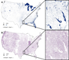 |
Fig. 1 Freshwater raster templates within the contiguous United States for (A) lakes (playas, lakes and ponds, certain reservoirs, and freshwater wetlands) and (B) streams (streams and rivers, canals and ditches, and connector channels) including the contiguous United States and zoomed into and area in Louisiana to illustrate local details. |
2.3 Environmental predictor data sources
We selected a suite of potential environmental predictors through a process of literature review and informal discussions with freshwater species researchers and managers about freshwater species in the northeast United States We filtered this list of potential predictors by considering relevant life-history characteristics of fish, plants, and invertebrates in streams and lakes. We further reduced the predictor set based on data availability or the ecological plausibility of creating a proxy from terrestrial data sources.
When in-stream or lake aquatic habitat predictors (such as water temperature or substrate) are unavailable, landscape predictors can serve as proxies for understanding and predicting aquatic habitat conditions. There is a long history of assessing aquatic habitat through the use of terrestrial proxies where aquatic environmental data are not available or are geographically restricted (Wiens, 2002; Allan, 2004). The landscape predictors can represent complex, and sometimes multi-factor influences to the aquatic habitat. For example, urban land use can indicate increased runoff, pollution, and altered stream hydrology (Paul and Meyer, 2001).
We obtained mean bioclimatic data for current conditions (1981–2010) and future projections (2011–2040) from the CHELSA 2.1 dataset (Karger et al., 2017; Karger et al., 2021). Future climate layers consist of five global circulation models of the shared socioeconomic pathway 370 (SSP370) from present to mid-century. The layers include 19 bioclimatic predictors, and other climatic metrics relevant to biological niches such as temperature extremes, potential water deficits, cumulative precipitation, and evapotranspiration (Tab. 1).
As a substitute for the lack of publicly available, geographically continuous, and comprehensive spatial datasets describing water chemistry characteristics, we used gridded soils data (which interpolate the physical and chemical properties of the terrestrial landscape (Nauman et al., 2017; Nauman et al., 2024]) to capture soil chemistry characteristics known to influence water chemistry (Fennessy and Cronk, 1997). We chose to use the HUC12 surrounding the lake or stream reach as the predictor resolution and processed using the zonal() function in the ‘terra’ package (Tab. 1). We chose these polygons to represent the resolution of our terrestrial proxy predictors, to capture how runoff impacts aquatic habitats, in addition to the predictor resolution representing the stream reaches or lakes themselves. As a result, the terrestrial-derived predictor layers represent single values for lakes and stream reaches, as processed from the surrounding landscape delineated by HUC12. For soil data, we calculated the mean of the raster values in HUC12 in which each pixel fell.
Using DEM data we calculated land slope and Multi-Scale Topographic Position Index (mTPI), a metric of topographic diversity, to capture the behavior of water on the landscape, particularly regarding runoff (Theobald et al., 2015). We also obtained current (2023) and forecasted (2050) (IPCC SRES A2 mid-century) land use and land cover layers to derive the proportion of cropland, grassland, forest, and developed land in landscapes surrounding freshwater habitats (Sohl et al., 2014; Sohl et al., 2018). We selected these land use and land cover categories for use as terrestrial proxies for water chemistry known to affect aquatic species. For example, habitat suitability for freshwater species can be influenced in highly disturbed lakes that are eutrophic due to fertilized agricultural runoff which affects the concentrations and ratios of nitrogen and phosphorus in the water (Chase and Knight, 2006; Zhang et al., 2022). Information about crop land cover, rainfall quantities and seasonality, slope, and soil characteristics that affect runoff can be used to capture the conditions that result in highly eutrophic lakes. Terrestrial land use proxies have been used to characterize water chemistry and stream habitat quality (Maloney and Weller, 2011; Katsiapi et al., 2012; Martinuzzi et al., 2014). Similar to soil data, because these are proxies for effects in freshwater from the surrounding landscape, we calculated the percent of cells of a given land cover category within the entire HUC12 polygon. Direct measurements of lakes consisted of lake shore area ratio (shore length / lake area provides shoreline density) from the NHD+ V2 HR dataset. We also derived seasonal metrics of mean streamflow and base flow index for current and future climate conditions for streams (USDA Forest Service, 2022).
2.4 Hydrological predictor estimation
Unique hydrological predictors were generated for each aquatic habitat model. For lake models, we calculated a shoreline density metric, or shore area ratio, by dividing the perimeter of the polygon by the area within the polygon using features already described in the NHD+ V2 HR dataset, to represent shoreline complexity. For stream models, we generated stream flow predictor layers for current and future flow scenarios utilizing existing flow discharge datasets. To generate current-period streamflow for all river segments, we used the mean annual flow estimates (1971–2000) provided for each NHDFlowline in the NHD+ V2 HR network used to define stream habitats. These values, measured in cubic feet per second, represent modeled discharge associated with each flowline segment. While flow values were linked to the NHDFlowline feature,the NHDFlowline multiline object and the NHDArea multipolygon object, representing wide rivers as polygons rather than lines, are used to define stream habitats. As such, a methodological challenge was that multiple NHDFlowline segments can intersect the same NHDArea polygon. To allocate flow values across these wide-river polygons, we identified all NHDFlowline segments intersecting each NHDArea polygon and calculated the midpoint of each intersecting segment. We then partitioned each NHDArea polygon into Voronoi sub-polygons based on equal distance from each line midpoint using the voronoi() function in the ‘terra’ R package (Hijmans, 2024) and assigned each flowline value to its corresponding Voronoi sub-polygon. This procedure ensured that flow values were accurately distributed across the full width of large rivers represented in the NHDArea polygons. All processing was conducted in parallel by HUC4, generating 212 rasters that were combined using the mosaic() function in the ‘terra’ R package (Hijmans, 2024). To generate our future stream flow predictor layer, we used the Hydro Flow Metrics for the Contiguous United States Absolute Change by Mid-Century dataset (USDA Forest Service, 2022). These estimates were generated by the Forest Service using historically modeled streamflow, future discharge projections for mid-century conditions (2040–2059) from five CMIP5 climate scenarios, the NHD+ V2 MR network (U.S. Geological Survey, 2019), and methods described by Wenger et al., 2010. We generated an absolute change layer using the same workflow applied to generate the current flow layer, including the Voronoi-based spatial allocation across NHDFlowline and NHDArea features. Processing was again performed by HU4 in parallel, generating 212 rasters that were combined using the mosaic() function. This parallel processing approach produced an absolute-change layer that matched the spatial structure, resolution, and formatting of the current-layer raster, allowing us to apply the delta method (Sofaer et al., 2017) to generate our future streamflow predictor layer. Although the older NHD+ V2 MR version does not include all flowlines present in NHD+ V2 HR dataset used to define stream habitats and current streamflow, this method yielded future estimates for the majority of modeled river segments in the HR dataset, with most missing segments corresponding to low-order headwater streams.
2.5 Final dataset development
We created a final dataset for lakes and one for streams by restricting each layer considered for the freshwater system (refer to Tab. 1) to the associated template rasters (e.g., lake layers to lake template, stream layers to stream template) with the mask() function in the ‘terra’ package. In these final layers, only cells in lakes for the lake dataset or streams for the stream dataset retained values, leaving the remaining land or freshwater areas with no data values. Finally, we standardized all GeoTIFFs to the same cell size, projection (ERSI:102008; NAD 1983 Albers North America), and extent using the ‘PARC’ (project, aggregate, resample, clip) module in the Software for Assisted Habitat Modeling (SAHM; Morisette et al., 2013). The final dataset contains 41 predictors calculated for both lakes and streams, with one additional lake predictor and two additional stream predictors (Tab. 1).
2.6 Data availability
These data, including the two template layers and raster layers described in Table 1 and associated code and metadata, are publicly available in Henderson et al. (2026).
Predictor data layers included in the national aquatic spatial dataset, where Processing Steps letter designations are A – PARC (Project-Aggregate-Resample-Clip) process to match the template, B- Summarized by Hydrologic Unit Code 12 (HUC12), C-Summarized by stream reach, D. All predictors were generated for both lakes and streams except mean annual stream flow and slope (stream only) and shore area ratio (lake only).
Predictor layers selected from the suite in Table 1 for inclusion in either the lake or stream models fit for Alternanthera philoxeroides, where an “X” indicates the predictor was offered to the model. (SD NDMI = standard deviation normalized difference moisture index; mTPI = multi-scale topographic position index).
3 Technical validation
3.1 Performance evaluation
To validate the performance of the national environmental data layers, we present a use-case for habitat suitability models constructed using these layers as environmental predictors for Alternanthera philoxeroides (Mart.) Griseb., commonly known as alligatorweed, an invasive aquatic plant in the southeastern United States (Thayer and Pfingsten, 2025). While the example we present is for an invasive aquatic plant species, the same methodology would be applicable for any freshwater species. We followed the methodology from the Invasive Species Habitat Tool (INHABIT) to generate occurrence models of terrestrial invasive plant species in CONUS (Jarnevich et al., 2024). Occurrence data were pulled from multiple publicly available sources in Jarnevich et al., 2024, with the addition of the Nonindigenous Aquatic Species database (U.S. Geological Survey, 2024). We filtered occurrence points into two sets using the lake template (n = 870) and the stream template (n = 782), selecting occurrences that fell within each of the templates. We selected predictors based on ecological knowledge of the species (Tab. 2). We fit models using the five algorithms within SAHM (boosted regression trees, generalized linear models, multivariate adaptive regression splines, Maxent, and random forests) with the occurrence data, target background points following Phillips et al., 2009, using occurrences of other non-native aquatic plant species, and the selected predictors. We produced maps by applying the model for each algorithm for lakes and the model for streams to both current and future prediction, producing an ensemble by calculating the mean prediction weighted by the continuous Boyce index (CBI; Hirzel et al., 2006) across model algorithms. We calculated the CBI, which ranges from −1 to 1 with 0 being the same as random, for the ensemble current lake and current stream models using a set of spatially withheld validation locations. The CBI score for lakes was 0.99 (0.96 train data) and for streams was 0.96 (0.96 train data), indicating that the habitat suitability models generated for alligatorweed using our suite of environmental predictors performed well. All model inputs and outputs are available in Jarnevich et al., 2026. We also examined the models for ecological plausibility based on species knowledge of experts, and it also met these expectations. Finally, we combined lake and stream maps to produce a single predicted freshwater suitable habitat for the species for both current and mid-century conditions and also calculated the difference between the two (Fig. 2). Most locations had values from only one model (lake or stream), but when there was a value in each, we calculated the mean of the predicted suitability.
For the development of habitat suitability models for organisms found in both lake and stream habitats, we provide data to develop a separate model for each habitat (lakes and streams) because there are some predictors specific to each habitat and different factors may be important in the different habitats. We provide an example where we created these individual models and then combined the prediction maps for the two habitat types for a single species within both habitat types.
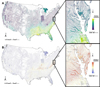 |
Fig. 2 Predicted suitable habitat for Alternanthera philoxeroides for (A) current environmental conditions and (B) predicted change in suitability for mid-century environmental conditions for the contiguous United States and zoomed into the Chesapeake Bay to illustrate local details. |
Acknowledgments
This research was supported by the U.S. Geological Survey, as part of a grant supplied by the Northeast Climate Adaptation Science Center. The authors would like to thank Anthony J. Martinez for his assistance in the development of the midpoint-voronoi methodology which enabled the creation of the data layers for stream habitats. Any use of trade, firm, or product names is for descriptive purposes only and does not imply endorsement by the U.S. Government.
Supplementary Material
Supplemental Table 1. Description of the National Hydrography Dataset (NHD) Plus High Resolution (HR) data products available and those used in predictor generation. Access Supplementary Material
References
- Abatzoglou JT. 2013. Development of gridded surface meteorological data for ecological applications and modelling. Int J Climatol 33: 121–131. [Google Scholar]
- Allan JD. 2004. Influence of land use and landscape setting on the ecological status of rivers. Limnetica 23: 187–197. [Google Scholar]
- Amatulli G, Garcia Marquez J, Sethi T, Kiesel J, Grigoropoulou A, Üblacker MM, Shen LQ, Domisch S. 2022. Hydrography90m: a new high-resolution global hydrographic dataset. Earth Syst Sci Data 14: 4525–4550. [Google Scholar]
- Buffagni A, Armanini DG, Erba S. 2009. Does the lentic-lotic character of rivers affect invertebrate metrics used in the assessment of ecological quality? J Limnol 68: 92–105. [Google Scholar]
- Chase JM, Knight TM. 2006. Effects of eutrophication and snails on Eurasian watermilfoil (Myriophyllum spicatum) invasion. Biol Invasions 8: 1643–1649. [Google Scholar]
- Domisch S, Jähnig SC, Simaika JP, Kuemmerlen M, Stoll S. 2015. Application of species distribution models in stream ecosystems: the challenges of spatial and temporal scale, environmental predictors and species occurrence data. Fund Appl Limnol 186: 45–61. [Google Scholar]
- Dudgeon D, Arthington AH, Gessner MO, Kawabata Z-I, Knowler DJ, Lévêque C, Naiman RJ, Prieur-Richard A-H, Soto D, Stiassny MLJ, Sullivan CA. 2006. Freshwater biodiversity: importance, threats, status and conservation challenges. Biol Rev 81: 163–182. [CrossRef] [PubMed] [Google Scholar]
- Elith J, Leathwick JR. 2009. Species distribution models: ecological explanation and prediction across space and time. Annu Rev Ecol Evol Syst 40: 677–697. [Google Scholar]
- Farr TG, Rosen PA, Caro E, Crippen R, Duren R, Hensley S, Kobrick M, Paller M, Rodriguez E, Roth L, Seal D, Shaffer S, Shimada J, Umland J, Werner M, Oskin M, Burbank D, Alsdorf D. 2007. The shuttle radar topography mission. Rev Geophys 45: RG2004. [Google Scholar]
- Fennessy MS, Cronk JK. 1997. The effectiveness and restoration potential of riparian ecotones for the management of nonpoint source pollution, particularly nitrate. Crit Rev Environ Sci Technol 27: 285–317. [Google Scholar]
- Forsyth DK, Riseng CM, Wehrly KE, Mason LA, Gaiot J, Hollenhorst T, Johnston CM, Wyrzykowski C, Annis G, Castiglione C, Todd K, Robertson M, Infante DM, Wang L, McKenna JE, Whelan G. 2016. The great lakes hydrography dataset: consistent, binational watersheds for the Laurentian Great Lakes basin. J Am Water Resour Assoc 52: 1068–1088. [Google Scholar]
- Guisan A, Thuiller W, Zimmermann NE. 2017. Habitat suitability and distribution models: with applications in R. C.U.P. [Google Scholar]
- Henderson G, Williams DA, Shadwell KS, Reimer CJ, LeClare SK, Fraser LS, Engelstad PS, Jarnevich CS. 2026. Freshwater habitat environmental predictor layers for waterbodies and streams across the contiguous United States: U.S. Geological Survey data release. https://doi.org/10.5066/P14JDTTJ. [Google Scholar]
- Hijmans RJ, Bivand R, Cordano E, Dyba K, Pebesma E, Sumner MD. 2024. terra: spatial data analysis (Version 1.7-83) [Computer software]. https://cran.r-project.org/web/packages/terra/index.html [Google Scholar]
- Hirzel AH, Le Lay G, Helfer V, Randin C, Guisan A. 2006. Evaluating the ability of habitat suitability models to predict species presences. Ecol Model 199: 142–152. [Google Scholar]
- Irving K, Kuemmerlen M, Kiesel J, Kakouei K, Domisch S, Jähnig SC. 2018. A high-resolution streamflow and hydrological metrics dataset for ecological modeling using a regression model. Sci Data 5: 180224. [Google Scholar]
- Jarnevich CS, Engelstad P, Williams D, Shadwell K, Reimer C, Henderson G, Prevey JS, Pearse IS. 2024. Predicted occurrence and abundance habitat suitability of invasive plants in the contiguous United States: updates for the INHABIT web tool. NeoBiota 96: 261–278. [Google Scholar]
- Jarnevich CS, Engelstad P, Williams DA, Shadwell KS, Reimer CJ, Henderson GC, Fraser L, LeClare S, Inman RD, Pfingsten I, Daniel W. 2026. Aqua INHABIT species potential distribution across the contiguous United States: U.S. Geological Survey data release. https://doi.org/10.5066/P13JMOQW. [Google Scholar]
- Jones KA, Niknami LS, Buto SG, Decker D. 2022. Federal standards and procedures for the national Watershed Boundary Dataset (WBD) (5 ed.): USGS Techniques and Methods 11-A3, 54 p. https://pubs.usgs.gov/tm/11/a3/ [Google Scholar]
- Karger DN, Conrad O, Böhner J, Kawohl T, Kreft H, Soria-Auza RW, Zimmermann NE, Linder HP, Kessler M. 2021. Data from: climatologies at high resolution for the earth's land surface areas. Envi Dat https://doi.org/10.16904/envidat.228.v2.1. [Google Scholar]
- Karger DN, Conrad O, Böhner J, Kawohl T, Kreft H, Soria-Auza RW, Zimmermann NE, Linder HP, Kessler M. 2017. Climatologies at high resolution for the earth's land surface areas. Sci Data 4: 170122. [Google Scholar]
- Katsiapi M, Mazaris AD, Charalampous E, Moustaka-Gouni M. 2012. Watershed land use types as drivers of freshwater phytoplankton structure. Hydrobiologia 698: 121–131. [Google Scholar]
- Kennedy RE, Yang Z, Gorelick N, Braaten J, Cavalcante L, Cohen WB, Healey S. 2018. Implementation of the LandTrendr Algorithm on Google Earth Engine. Remote Sens 10: Article 5. [Google Scholar]
- Maloney KO, Weller DE. 2011. Anthropogenic disturbance and streams: land use and land use change affect stream ecosystems via multiple pathways: Land use affects streams via multiple pathways. Freshw Biol 56: 611–626. [Google Scholar]
- Martinuzzi S, Januchowski-Hartley SR, Pracheil BM, McIntyre PB, Plantinga AJ, Lewis DJ, Radeloff VC. 2014. Threats and opportunities for freshwater conservation under future land use change scenarios in the United States. Glob Change Biol 20: 113–124. [Google Scholar]
- McGarvey DJ, Menon M, Woods T, Tassone S, Reese J, Vergamini M, Kellogg E. 2018. On the use of climate covariates in aquatic species distribution models: are we at risk of throwing out the baby with the bath water? Ecography 41: 695–712. [Google Scholar]
- Moore RB, McKay LD, Rea AH, Bondelid TR, Price CV, Dewald TG, Johnston CM. 2019. User's guide for the national hydrography dataset plus (NHDPlus) high resolution. In Open-File Report (Nos. 2019–1096). USGS. https://doi.org/10.3133/ofr20191096 [Google Scholar]
- Morisette JT, Jarnevich CS, Holcombe TR, Talbert CB, Ignizio DA, Talbert M, Silva C, Koop D, Swanson A, Young NE. 2013. VisTrails SAHM: Visualization and workflow management for species habitat modeling. Ecography 36: 129–135. [Google Scholar]
- Nauman TW, Kienast-Brown S, Roecker SM, Brungard C, White D, Philippe J, Thompson JA. 2024. Soil landscapes of the United States (SOLUS): developing predictive soil property maps of the conterminous United States using hybrid training sets. Soil Sci Soc Am J 88: 2046–2065. [Google Scholar]
- Nauman T, Ramcharan A, Brungard C, Thompson J, Wills S, Waltman S, Hengl T. 2017. Soil properties and class 100m grids united states [dataset]. https://doi.org/10.18113/S1KW2H [Google Scholar]
- Nori J, Rojas-Soto O. 2019. On the environmental background of aquatic organisms for ecological niche modeling: a call for caution. Aquat Ecol 53: 595–605. [Google Scholar]
- Paul MJ, Meyer JL. 2001. Streams in the urban landscape. Annu Rev Ecol Syst 32: 333–365. [CrossRef] [Google Scholar]
- Phillips SJ, Dudík M, Elith J, Graham CH, Lehmann A, Leathwick J, Ferrier S. 2009. Sample selection bias and presence-only distribution models: Implications for background and pseudo-absence data. Ecol Appl 19: 181–197. [CrossRef] [PubMed] [Google Scholar]
- R Core Team. 2025. R: A language and environment for statistical computing. [Computer software]. R Foundation for Statistical Computing. https://www.R-project.org/ [Google Scholar]
- Ross MRV, Topp SN, Appling AP, Yang X, Kuhn C, Butman D, Simard M, Pavelsky TM. 2019. AquaSat: a data set to enable remote sensing of water quality for inland waters. Water Resour Res 55: 10012–10025. [Google Scholar]
- Seaber PR, Kapinos FP, Knapp GL. 1987. Hydrologic unit maps. https://doi.org/10.3133/WSP2294 [Google Scholar]
- Senay GB, Bohms S, Singh RK, Gowda PH, Velpuri NM, Alemu H, Verdin JP. 2013. Operational evapotranspiration mapping using remote sensing and weather datasets: a new parameterization for the SSEB approach. J Am Water Resour Assoc 49: 577–591. [Google Scholar]
- Sofaer HR, Barsugli JJ, Jarnevich CS, Abatzoglou JT, Talbert MK, Miller BW, Morisette JT. 2017. Designing ecological climate change impact assessments to reflect key climatic drivers. Glob Change Biol 23: 2537–2553. [Google Scholar]
- Sofaer HR, Jarnevich CS, Pearse IS, Smyth RL, Auer S, Cook GL, Edwards TC, Jr, Guala GF, Howard TG, Morisette JT, Hamilton H. 2019. Development and delivery of species distribution models to inform decision-making. BioScience 69: 544–557. [Google Scholar]
- Sohl TL, Sayler KL, Bouchard MA, Reker RR, Friesz AM, Bennett SL, Sleeter BM, Sleeter RR, Wilson T, Knuppe M, Van Hofwegen T. 2018. Conterminous United States land cover projections—1992 to 2100 [Dataset]. USGS. https://doi.org/10.5066/P95AK9HP [Google Scholar]
- Sohl TL, Sayler KL, Bouchard MA, Reker RR, Friesz AM, Bennett SL, Sleeter BM, Sleeter RR, Wilson T, Soulard C, Knuppe M, Van Hofwegen T. 2014. Spatially explicit modeling of 1992–2100 land cover and forest stand age for the conterminous United States. Ecol Appl 24: 1015–1036. [Google Scholar]
- Thayer DD, Pfingsten IA. 2025. Alternanthera philoxeroides (Mart.) Griseb.: U.S. Geological Survey, Nonindigenous Aquatic Species Database, Gainesville, FL, https://nas.er.usgs.gov/queries/FactSheet.aspx?SpeciesID=227, Revision Date: 12/5/2024, Peer Review Date: 4/4/2016 [Google Scholar]
- Theobald DM, Harrison-Atlas D, Monahan WB, Albano CM. 2015. Ecologically-relevant maps of landforms and physiographic diversity for climate adaptation planning. PLOS ONE 10: e0143619. [Google Scholar]
- Theobald DM, Kennedy C, Chen B, Oakleaf J, Baruch-Mordo S, Kiesecker J. 2020. Earth transformed: detailed mapping of global human modification from 1990 to 2017. Earth Syst Sci Data 12: 1953–1972. [Google Scholar]
- U.S. Environmental Protection Agency. 2022. NARS Lake and Stream Predictor Dataset, V1 [Dataset]. U.S. EPA ORD. https://doi.org/10.23719/1528186 [Google Scholar]
- U.S. Geological Survey. 2019. National Hydrography Dataset (ver. USGS National Hydrography Dataset Best Resolution (NHD) for Hydrologic Unit (HU) 4 - 2001 (published 20191002)), accessed 2024 at URL https://www.usgs.gov/national-hydrography/access-national-hydrography-products [Google Scholar]
- U.S. Geological Survey. 2022. USGS National Hydrography Dataset Plus High Resolution National Release 1 FileGDB [Dataset]. https://doi.org/10.5066/P9WFOBQI [Google Scholar]
- U.S. Geological Survey. 2024. Nonindigenous Aquatic Species Database, Gainesville, FL. http://nas.er.usgs.gov, 2024. [Google Scholar]
- USDA Forest Service. 2022. Flow Metrics for the Contiguous United States (Absolute Change by Mid-Century) [Dataset]. Accessed 8 July 2024 from https://data.fs.usda.gov/geodata/edw/datasets.php?xmlKeyword=hydro+flow+metric [Google Scholar]
- Wang L, Riseng CM, Mason LA, Wehrly KE, Rutherford ES, McKenna JE, Castiglione C, Johnson LB, Infante DM, Sowa S, Robertson M, Schaeffer J, Khoury M, Gaiot J, Hollenhorst T, Brooks C, Coscarelli M. 2015. A spatial classification and database for management, research, and policy making: The Great Lakes aquatic habitat framework. J Great Lakes Res 41: 584–596. [Google Scholar]
- Wenger SJ, Luce CH, Hamlet AF, Isaak DJ, Neville HM. 2010. Macroscale hydrologic modeling of ecologically relevant flow metrics. Water Resour Res 46. [Google Scholar]
- Wiens JA. 2002. Riverine landscapes: taking landscape ecology into the water. Freshw Biol 47: 501–515. [Google Scholar]
- Zhang Y, Leng Z, Wu Y, Jia H, Yan C, Wang X, Ren G, Wu G, Li J. 2022. Interaction between Nitrogen, Phosphorus, and Invasive Alien Plants. Sustainability 14: Article 2. [Google Scholar]
Cite this article as: Henderson GC, Engelstad P, Reimer CJ, Leclare SK, Fraser LS, Williams DA, Shadwell KS, Daniel WM, Pfingsten IA, Jarnevich CS. 2026. Current and near-future conditions of aquatic spatial data for use in ecological models in the United States. Knowl. Manag. Aquat. Ecosyst., 427, 11. https://doi.org/10.1051/kmae/2026003
All Tables
Predictor data layers included in the national aquatic spatial dataset, where Processing Steps letter designations are A – PARC (Project-Aggregate-Resample-Clip) process to match the template, B- Summarized by Hydrologic Unit Code 12 (HUC12), C-Summarized by stream reach, D. All predictors were generated for both lakes and streams except mean annual stream flow and slope (stream only) and shore area ratio (lake only).
Predictor layers selected from the suite in Table 1 for inclusion in either the lake or stream models fit for Alternanthera philoxeroides, where an “X” indicates the predictor was offered to the model. (SD NDMI = standard deviation normalized difference moisture index; mTPI = multi-scale topographic position index).
All Figures
|
Fig. 1 Freshwater raster templates within the contiguous United States for (A) lakes (playas, lakes and ponds, certain reservoirs, and freshwater wetlands) and (B) streams (streams and rivers, canals and ditches, and connector channels) including the contiguous United States and zoomed into and area in Louisiana to illustrate local details. |
| In the text | |
|
Fig. 2 Predicted suitable habitat for Alternanthera philoxeroides for (A) current environmental conditions and (B) predicted change in suitability for mid-century environmental conditions for the contiguous United States and zoomed into the Chesapeake Bay to illustrate local details. |
| In the text | |
Current usage metrics show cumulative count of Article Views (full-text article views including HTML views, PDF and ePub downloads, according to the available data) and Abstracts Views on Vision4Press platform.
Data correspond to usage on the plateform after 2015. The current usage metrics is available 48-96 hours after online publication and is updated daily on week days.
Initial download of the metrics may take a while.