| Issue |
Knowl. Manag. Aquat. Ecosyst.
Number 421, 2020
|
|
|---|---|---|
| Article Number | 31 | |
| Number of page(s) | 13 | |
| DOI | https://doi.org/10.1051/kmae/2020024 | |
| Published online | 14 July 2020 | |
Research Paper
Ecosystems of artificial saline lakes. A case of Lake Magic in Wadi El-Rayan depression (Egypt)
Ecosystèmes de lacs salés artificiels. Le cas du lac magique dans la dépression de Wadi El-Rayan (Égypte)
1
A.O. Kovalevsky Institute of Biology of the Southern Seas of RAS, 299011 Sevastopol, Russia
2
National Institute of Oceanography and Fisheries, Cairo, Egypt
* Corresponding author: This email address is being protected from spambots. You need JavaScript enabled to view it.
, This email address is being protected from spambots. You need JavaScript enabled to view it.
Received:
17
May
2020
Accepted:
10
June
2020
Abstract
The Wadi El-Rayan is a depression in the Fayoum oasis collecting agricultural drainage water from the Fayoum. Since 1973, this drainage water formed two man-made lakes. Twenty years ago, a third lake, called Lake Magic was formed. Since this newly formed lake was not yet studied, in January of 2019 we conducted research related to its physico-chemical (ion composition, nutrients, heavy metals, etc.) and biological (phyto-, bacterio- and zooplankton) characteristics. The depth of the lake ranged from 1.5 to 9.0 m, water transparency was up to 4.0 m, and the water temperature was 13.6 °C. The average salinity was 29.1 g/l, and the salinity of drainage waters from agricultural fields was 2.9 g/l. A total of 28 phytoplankton species was identified belonging to Bacillariophyceae (eight species), Dinophyceae (three species), Cyanobacteria (seven species), Chlorophyceae (nine species) and Conjugatophyceae (one species). Chlorophyll a content varied from 14.3 to 24.2 μg/l. In zooplankton, there were three species of Ciliophora, five of Rotifera, and two Copepoda as well as Nematoda and Cirripedia larvae. Salinity in Lake Magic was much higher than in drainage waters coming in the lake. This is a result of a strong salinity increase in Lake Magic after its creation due to climate aridity, and salinity may markedly increase during the next 20 years along with the sharp changes of the lake's ecosystem.
Résumé
Le Wadi El-Rayan est une dépression dans l'oasis du Fayoum qui recueille les eaux de drainage agricole du Fayoum. Depuis 1973, ces eaux de drainage ont formé deux lacs artificiels. Il y a vingt ans, un troisième lac, appelé Lac magique, s'est formé. Comme ce lac nouvellement formé n'était pas encore étudié, nous avons mené en janvier 2019 des recherches sur ses caractéristiques physico-chimiques (composition ionique, nutriments, métaux lourds, etc.) et biologiques (phyto-, bactério- et zooplancton). La profondeur du lac variait de 1,5 à 9,0 m, la transparence de l'eau atteignait 4,0 m et la température de l'eau était de 13,6 ᵒC. La salinité moyenne était de 29,1 g/l, et la salinité des eaux de drainage des champs agricoles était de 2,9 g/l. Au total, 28 espèces de phytoplancton ont été identifiées, appartenant aux catégories suivantes : Bacillariophyceae (huit espèces), Dinophyceae (trois espèces), Cyanobactéries (sept espèces), Chlorophyceae (neuf espèces) et Conjugatophyceae (une espèce). La teneur en chlorophylle a varié de 14,3 à 24,2 μg/l. Dans le zooplancton, il y avait trois espèces de Ciliophora, cinq de Rotifera, et deux Copepoda ainsi que des larves de Nematoda et de Cirripedia. La salinité du lac magique était beaucoup plus élevée que celle des eaux de drainage provenant du lac. Ceci est le résultat d'une forte augmentation de la salinité du lac magique après sa création en raison de l'aridité du climat, et la salinité pourrait augmenter sensiblement au cours des 20 prochaines années en même temps que les changements importants de l'écosystème du lac.
Key words: man-made lakes / arid areas / salinization / ecosystems / long-term changes
Mots clés : lacs artificiels / zones arides / salinisation / écosystèmes / changements à long terme
© E.V. Anufriieva et al., Published by EDP Sciences 2020
 This is an Open Access article distributed under the terms of the Creative Commons Attribution License CC-BY-ND (https://creativecommons.org/licenses/by-nd/4.0/), which permits unrestricted use, distribution, and reproduction in any medium, provided the original work is properly cited. If you remix, transform, or build upon the material, you may not distribute the modified material.
1 Introduction
Human activities have changed ecosystems and landscapes since prehistoric times. One of the examples is a transformation of the existing natural saline lakes into the hybrid natural and technological water bodies which creates the new artificial saline lakes (Hammer, 1986; Han and Park, 1999; Kurlansky, 2002; Shadrin et al., 2012). The most common cases of hybrid natural and technological saline lakes are natural lakes that are separated on several parts, with their salinities regulated by humans for technological or medical needs. The first such system for salt production, Lake Yuncheng, is known from China originating from more than 5000 years ago (Kurlansky, 2002). Construction, hydromelioration, mining, and other human activities may lead to the formation of artificial saline lakes (Hammer, 1986; Han and Park, 1999; Shadrin et al., 2012). Irrigation with drainage water discharge from agricultural fields into depressions is a specific cause of artificial lake origin in the arid areas. The best known example is the Salton Sea in the USA, which is also the largest artificial saline lake (area 930–1000 km2) in the world (Hely et al., 1966; Schroeder et al., 2002). Lake Qarun (Egypt) is likely the oldest case of an artificial or hybrid between the natural and man-made lakes (Hassan, 1986). The Canal Bahr Yousef was constructed in early Pharaonic times, i.e., earlier than 2500 BC to provide fresh water from the River Nile to agricultural fields in the desert areas (Hassan, 1986). The Canal branches out, providing water to agricultural lands in the Fayoum (Faiyum) oasis, which is the desert basin to the west of the Nile and south of Cairo. Drainage water discharge slowly formed Lake Qarun, which contained freshwater for a long-time, but then it transformed into the high saline lake due to climate aridity (El-Shabrawy et al., 2015; Shadrin et al., 2016). Man-made water bodies significantly change the system of landscape connections. Not infrequently they may be valuable for biodiversity conservation as they can provide habitat for many species, highly increasing local biodiversity, especially of birds (Shuford et al., 2002; El-Shabrawy and Dumont, 2009; Downing, 2010; Voyles, 2016; Vilenica et al., 2020). They also create a new opportunity for the development of various types of human activities including recreation, tourism, fishing, aquaculture, chemical industry, etc. (Black, 1988; El-Shabrawy and Dumont, 2009; Ramzy, 2013; Anufriieva, 2018; Shalloof, 2020). Due to climate aridity and human activities, in some man-made lakes, the salinity can gradually fluctuate and increase, which along with ecosystem changes, create a lot of the problems for people and their activities (Hussein et al., 2008; Cohen, 2009; Afefe et al., 2016; Shadrin et al., 2016; Voyles, 2016; Shalloof, 2020).
Current science is far from being able to predict possible changes in man-made saline lakes to the point of preventing or mitigating unwanted events. Since man-made lakes make up at least half of small lakes and ponds, the global role of small lakes and ponds emerges as an important area of investigation (Downing, 2010). Taking this into account, we suggest that the development of the tools to predict the future dynamics of artificial saline lakes is a high priority. Only by accumulating a critical volume of data on changes of such lakes, can researchers move towards developing effective tools to forecast the response of these lakes to ecosystem changes. With the main aim to increase our knowledge about physico-chemical and biological characteristics of artificial saline lakes, we conducted a study of the completely unknown Lake Magic in Egypt. The main goals were: (i) to investigate physico-chemical and biological characteristics of the lake, (ii) to analyze interrelation between different characteristics and homogeneity of their spatial distribution, (iii) to develop the possible forecast of the future lake changes.
2 Materials and methods
2.1 Study area
Wadi El-Rayan (1759 km2, 29°17′N, 30°23′E) is a natural desert depression in the Fayoum Oasis, 42–60 m below the sea level, connected with the agricultural drainage water system of the Fayoum depression (Maiyza et al., 1999; El-Shabrawy and Dumont, 2009; El Gammal and El Gammal, 2010). Before the Aswan High Dam construction on the River Nile, only Lake Qarun served as a reservoir for agricultural drainage water from irrigated agriculture in the Fayoum depression. As a result of the dam construction, the drainage water volume consequently increased creating a dangerous risk (Mayza et al., 1999). To mitigate the problem, the Wadi El-Rayan Project was developed. Since 1973, the agricultural wastewater drainage through the El-Wadi Drain was started in an uninhabited depression, resulting in the formation of two man-made connecting lakes (El-Shabrawy and Dumont, 2009). The first (upper) lake covers about 53 km2 (10 m below the sea level) receiving about 200 million m3 of agricultural drainage water annually (Sayed and Abdel-Satar, 2009). From this lake, surplus water floods through the shallow connecting channel into the second lower lake. The lower lake is larger and occupies up to 110 km2 (18 m below the sea level) with a maximum depth of 33 m. The total capacity of these two lakes exceeds the capacity of Lake Qarun. This lake has increased its area, flooding new areas, and adding territory on the southwestern side (El-Shabrawy and Dumont, 2009; El Gammal and El Gammal, 2010). The Wadi El-Rayan area was designated as a Protected Area in 1989 to protect the biological, geological and cultural diversity. Two man-made lakes, which connected by a swampy channel, were designated as Ramsar wetlands in 2012. Now sabkhas, sand flats, dunes, wetlands (man-made lakes), three natural springs are the main types of habitats in the depression. Contrary to most desert areas, the depression holds a high biological diversity, and man-made saline lakes contribute to this. This region has continued to develop, with the construction of villages, agriculture, fisheries, and aquaculture (fish farming) (El-Shabrawy and Dumont, 2009; El Gammal and El Gammal, 2010; Goher et al., 2019). In 1998–1999, as a result of land reclamation and construction of some new villages in the Wadi El-Rayan, a third lake was formed called Lake Magic situated about 65 km southwest of Fayoum city (Fig. 1). It lies about 2.7 km to the west of the second (lower) Rayan Lake. Lake Magic was named because it magically changes colors several times every day depending on day time and amount of sunlight (Egypt Today, 2017). This terminal lake does not have any connection with the other two lakes in the depression. This newly formed lake occupies about 0.42 km2, with a length of 1200 m, a width of 350 m, and a max depth of 9 m. With a planned increase in agricultural discharge, it is expected to reach an area of more than 0.63 km2 and a max depth of 12 m. The source of water for the Lake Magic is a drain (minor canal) facing sampling station 8 (Fig. 1) that collects the agriculture drainage from the neighboring land of the new villages (El-Walaa and Kheder). According to information obtained from the local citizens, irrigated agricultural fields occupy around 11 km2, and most important crops are olives, followed by Phoenix palms, alfalfa, tomatoes, and broad bean. It is significantly smaller than the two older lakes but is also very important for the local population, including fishery, aquaculture, and tourism. Although there have been some studies conducted on the first two lakes (Maiyza et al., 1999; El-Shabrawy and Dumont, 2009; El Gammal and El Gammal, 2010; Goher et al., 2019), there is no published study on Lake Magic. Therefore, in January 2019, we conducted the first study at 10 stations along the lake (Fig. 1).
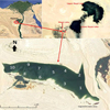 |
Fig. 1 Lake Magic location and distribution of the sampling sites. |
2.2 Physical and chemical water properties
In January 2019, water samples were collected at ten stations along the lake (Fig. 1, Tab. 1), using a polyvinyl chloride Van Dorn bottle water sampler with a volume of 2 l. Dissolved oxygen (DO) was measured by immediately fixing the water with 1 ml MnSO4 (40%) and 1 ml alkaline KI solution, while the bottles for measuring biochemical oxygen demand (BOD) were covered by aluminum foil and incubated at 20 °C. Water temperature, electrical conductivity, and pH value were measured in situ, using hydro-lab model Orion Research Ion Analyzer 399A (ORION Research Inc., Cambridge, Massachusetts, USA). The transparency was measured using the Secchi-disk with a diameter of 30 cm. Water samples were kept in 2 l polyethylene bottles in an icebox and analyzed in the laboratory. Water chemistry analyses were carried out according to the APHA standard methods (2005). The following parameters were measured: TS (total solids), TDS (total dissolved solids), TSS (total suspended substances), DO (dissolved oxygen), BOD (biological oxygen demand), COD (chemical oxygen demand), water alkalinity (carbonate and bicarbonate), calcium, magnesium, NO2-N, NO3-N, NH4-N, PO4-P, SiO4, TP (total phosphorus), and TN (total nitrogen). Na+, K+, were measured directly using the flame photometer model Jenway PFP-7 (Bibby Scientific Ltd., Stone, UK). The concentration of heavy metals was measured after digestion by concentrated HNO3 using the GBC atomic absorption reader model Savant AA-AAS with GF 5000 graphite furnace (GBC Scientific Equipment Rty Ltd, Braeside, Australia).
Coordinates and some characteristics of sampling sites in Magic Lake during January 2019.
2.3 Phytoplankton
For the phytoplankton examination, upper layer water sampling was collected at the same ten stations. At each station, one liter of water was preserved with 4% formalin and Lugols iodine immediately. The samples were transported in the glass cylinders into the laboratory, and conserved for 5 days. Approximately, 90% of the supernatant was siphoned off by plastic tubes protected with plankton mesh of 55 μm, and adjusted to a stable volume. One quantitative sample was collected from each site, each site sample was divided into three sub-samples and each sub-sample was analyzed separately. The net result is the mean of the three subsamples results. Sub-samples were prepared for species identification and account using an inverted microscope. Each sample was examined and enumerated via a drop method (APHA, 2005). Various identification tools were used for phytoplankton species identification (Huber-Pestalozzi, 1961, 1983; Komárek and Anagnostidis, 1986, 1989, 1999; Krammer and Lange-Bertalot, 1986, 1988, 1991a, 1991b; Anagnostidis and Komárek, 1988; Popovský and Pfiester, 1990).
2.4 Chlorophyll a
A known volume of water (50 ml of triplicate subsamples) was filtered in situ on glass microfiber filter GF/F, using the Sartorius filtration unit. The filter containing the filtrate was wrapped in aluminum foil and preserved in a dark icebox. In a laboratory, chlorophyll was extracted by socking the filter in 5 ml acetone (90%) and preserved in dark overnight at 20 °C. The samples were shaken well and centrifuged; the clear acetone extract was siphoned carefully then chlorophyll a was estimated by Jenway 6800 Double-Beam Spectrophotometer (Bibby Scientific Ltd, Staffordshire, UK) visible spectrophotometer using 90% acetone as blank. The concentrations of chlorophyll a were calculated according to the trichromatic equation (APHA, 2005).
2.5 Bacteriology
The water samples were collected at the same locations by using sterilized glass bottles. They were brought into laboratories and stored on ice in insulated containers. Bacteriological analyses of water samples were done using standard methods (APHA, 2005). One quantitative sample was collected from each site, each site sample was divided into three sub-samples and each sub-sample was analyzed separately. The net result is the mean of the three subsamples results. Sub-samples were analyzed for a total viable bacterial count and a total count of different bacterial indicators using the poured plates and the most probable number (MPN) technique, respectively. Poured plates technique: the method for decimal dilution of water samples was used for the determination of a total bacterial load, on nutrient agar. The plates were incubated for 1–2 days for fast growing bacteria at 37 °C and 2–3 days at 22 °C for characteristic water bacteria. MPN: The most probable number technique was carried out for the estimation of some microbial indicators in the tested water samples using special presumptive and confirmed tests for each indicator. During the presumptive test, 5 ml of each appropriate three decimal dilutions of raw water samples were used to inoculate five tubes, each containing 5 ml of proper medium (single strength), and the tubes were incubated at 37 °C for 48 hours. The positive presumptive tubes were used to inoculate the confirmed test which detected the bacterial indicators as following: (1) total coliform (TC); lauryl tryptose broth medium was used for the presumptive test. The positive tubes which showed gas and acid were used to inoculate brilliant green lactose bile broth medium (BGB), as a confirmed test. The production of gas and acid was recorded as a positive confirmed test for total coliforms. (2) Fecal coliform (FC) estimation was carried out by inoculation in the EC broth tubes from positive BGB broth medium tubes, then incubated at 44.5 °C for 24 hours. The positive tubes containing gas production were used to detect the count per 100 ml sample (MPN index/100 ml) and streak the eosin methylene blue agar medium (EMB) plates, then incubated at 37 °C for 24 hours. Metallic sheen colonies considered as a positive confirmed result for Escherichia coli presence. (3) Fecal streptococci (FS); azide dextrose broth was used as a presumptive test without fermentation tubes. The positive tubes were turbid, then used to inoculate ethyl violet azide broth medium as a confirmed test. The positive results were turbid after incubation at 37 °C for 48 hours.
2.6 Zooplankton
Zooplankton quantitative samples were collected from the surveyed stations by vertical net (55 μm mesh diameter) filtering of 50 l of water (in two replicates). Qualitative samples with large volume filtered were also taken for the detection of highly scarce and sporadic species. Samples were immediately preserved in 4% neutral formalin. One quantitative sample was collected from each site, each site sample was divided into three sub-samples and each sub-sample was determined separately. The net result is the mean of the three subsamples results. The major groups of zooplankton were subjected to detailed microscopic analysis and identification using the following identification tools (Rudescu, 1960; Yamaji, 1978; Al-Yamani et al., 2011; Conway, 2012a,b).
2.7 Data processing
Data were processed by standard statistical methods (Sokal and Rohlf, 1995). Average values, coefficients of correlations (R), determination (R 2), variability (CV) and standard deviation (SD), as well as parameters of regression equations, were calculated using the standard program MS Excel 2007. The significance of average value differences (p) was tested by Student's t-test with normality tests before this (Thode, 2002). The confidence level of R was evaluated by comparing with R critical values (p ≤ 0.05) (Müller et al., 1979). STATISTICA 6 was used to calculate Euclidean distances between stations in the cluster analysis. The frequency of different species occurring in the samples was calculated as a number of samples with a species/a total number of samples.
3 Results
3.1 General and physico-chemical characteristics
The lake's depth ranged from 1.5 to 9.0 m (average 3.3 m, SD = 2.20, CV = 0.663) between the sampling stations (Tab. 1). Water transparency extended to 4.0 m and was greater in the stations with depths of less than 3.5 m (Tab. 1). The average lake temperature was 13.6 °C (SD = 0.2, CV = 0.016) (Tab. 1). Average salinity was 29.1 g/l varying in a narrow range (SD = 0.15, CV = 0.01) (Tab. 2). During the sampling time, the salinity of drainage waters from agricultural fields was 2.9 g/l. Ion composition showed low variations between the sampling stations (Tab. 2). The proportion between main anions (Cl/SO4) was 1.38 (SD = 0.03, CV = 0.020). The performed cluster analysis using the data from Table 2 showed that all the stations break up into two main clusters, although the Euclidean distances between them are not very large (Fig. 2a). The first cluster included stations 1–7, and the second cluster included stations 8–9 (Fig. 2a). There is only one drainage water input into the lake, which is near the sampling station 8, and the nearest sampling stations (8, 9, 10) stand out as a separate group. Other obtained chemical characteristics of the aquatic environment, including the concentration of nutrients, are given in Table 3. The spatial variability of most characteristics is also extremely low; it was highest for PO4 (CV = 0.26), BOD (CV = 0.21) and NO3 (CV = 0.18). The average oxygen concentration is quite high, 8.6 mg/l, and not very variable (Tab. 3). According to the parameters of Table 3, the stations were divided into two main clusters, the same as above (Fig. 2a). Among all characteristics, TP and PO4 were only significantly different in 1st and 2nd clusters (p = 0.05–0.005); they were higher in the second one on 60 and 21%, respectively. The concentrations of the studied heavy metals are given in Table 4. The spatial variability of the heavy metal concentrations was on average higher, but not much than other abiotic characteristics of the medium. The smallest variability was observed for Fe (CV = 0.09), and the largest for Cu (CV = 0.26), Zn (CV = 0.24) and Cd (CV = 0.21). Cluster analysis with the data Table 3 showed that all stations were divided into two main groups (Figure 2b), which were not the same as the clusters in Figure 2a. The first cluster included the sampling points 1, 2, 6–10, and the second cluster included the sampling points 3–5. The concentration of three heavy metals significantly differed in these two groups of stations (p = 0.05), in the second group of stations (3, 4, and 5), the concentration of Fe and Zn was 1.2 and 1.5 times higher, respectively. The concentration of Cr in this group of stations was 1.2 times lower than in the other one.
Correlation analysis was done for all pairs of studied abiotic characteristics, whereas 26 significant correlations were found (Tab. 5). As an example, values of BOD and COD being quite high, significantly negatively correlated with each other (Tab. 5, Eq. (1)). PO4 amount significantly positively correlated with concentrations of Fe, Ca, and Cd (Tab. 5, Eqs. (6)–(8)). SO4 amount significantly positively correlated with concentrations of Ca and Cu (Tab. 5, Eqs. (12) and (13)). Depth significantly negatively correlated with concentrations of Zn and Pb (Tab. 5, Eqs. (18) and (19)). The depth affects the TSS: with an increase in depth up to 4.5 m, the TSS significantly decreases (R = ‑0.697, p = 0.01), and at a point with a depth of 9 m, it sharply increases to the maximum value.
Salinity and major cations and anions in Lake Magic during January 2019.
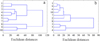 |
Fig. 2 Similarities between the sampling sites according different abiotic characteristics (a − clustering of sites according chemical characteristics from Tabs. 2 and 3; b − clustering of sites according heavy metals content characteristics from Tab. 4). |
Some hydrochemical characteristics in Magic Lake during January 2019.
Heavy metal concentrations in water of Magic Lake during January 2019.
Correlations between different chemical characteristics of water in Magic Lake during January 2019.
3.2 Phytoplankton and chlorophyll a
A total of 28 phytoplankton species was identified in Lake Magic during this study belonging to Bacillariophyceae (8 species), Dinophyceae (3 species), Cyanobacteria (7 species), Chlorophyceae (9 species) and Conjugatophyceae (1 species) (Tab. 6). The frequency of occurrence of different species in the samples varied from 10 to 80%. The number of species in a sample fluctuated from 5 to 18, and the highest values were in points 3 (18 species) and 5 (17 species). The lowest values were in points 9 (5 species) and 8 (7 species). The most distinct phytoplankton was that from station 5, where we also recorded the highest total phytoplankton abundance (1 × 10⁷ cells/l). The lowest abundance (9 × 10⁵ cells/l) was determined for station 10 (Fig. 3a, Tab. 6). The contribution of different taxa in total phytoplankton abundance varied from one sampling station to another (Tab. 6). Considering the abundance, Bacillariopyhceae and Dinophyceae dominated in three cases, and Cyanobacteria, in two cases. Bacillariopyhceae and Dinophyceae had the same abundance in one sample, as well as Cyanobacteria and Dinophyceae. Cluster analysis based on the contribution of different taxa to total phytoplankton abundance showed that all sampling stations were separated into two groups, with station 5 being different from both these groups (Fig. 3a). Station 5 had the highest contribution of Cyanobacteria (49%) in phytoplankton total abundance (Tab. 6).
Chlorophyll a content varied from 14.3 μg/l (station 10) to 24.2 μg/l (station 5) at majority of the sampling stations, with an average of 18.6 μg/l (CV = 0.179) (Fig. 4). At station 7, despite the lowest phytoplankton abundance, the chlorophyll a was 48.6 μg/l (Fig. 4a). If station 7 is excluded, there was significant positive correlation between phytoplankton abundance and chlorophyll a content (R = 0.765, p = 0.005) (Fig. 4b):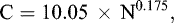 (1)
(1)
where C − chlorophyll a content, μg/l; N − cell abundance, 105 cell/l.
Species composition of phytoplankton in Magic Lake during January 2019.
 |
Fig. 3 Clustering of sites according phytoplankton (a), microbiological characteristics (b), zooplankton (c). |
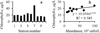 |
Fig. 4 Phytoplankton in Magic Lake during January 2019 (a − chlorophyll a distribution, b − correlation between chlorophyll a content and phytoplankton abundance). |
3.3 Bacteria
The numbers of aerobic bacteria (TVBC) at 22 °C ranged from 11 × 102 CFU/ml and 36 × 102 CFU/ml, while the bacteria developing (TVBC) at 37 °C varied from 22 × 102 CFU/ml to 75 × 102 CFU/ml (Fig. 5). The highest value at 22 °C was recorded at stations 4 and 8, while the highest value at 37 °C was recorded at station 5. Total coliform bacteria (TC), fecal coliform bacteria (FC) and fecal streptococci (FS) varied from station to station in a wide range (Tab. 7). The highest values of TC (150/100 ml) and FC (93 MPN/100 ml) were recorded at station 8, nearest to only single drainage input in the lake (Tab. 7). An abundance of FS numbers was in the range of 150–2900 MPN/100 ml, and the highest values of FS were recorded at stations 3 and 4 (Tab. 7). The lowest values of FC and FS were found at the deepest station, station 5.
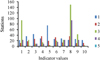 |
Fig. 5 Distribution of bacterial indicators in Lake Magic during January 2019 (1–TVBC at 37 °C, 102 CFU/m; 2–TVBC at 22 °C, 102 CFU/m; 3–TC, MPN/100 ml; 4–FC, MPN/100 ml; 5–FS, 102 MPN/100 ml). |
Microbiological characteristics in Magic Lake during January 2019.
3.4 Zooplankton
In zooplankton community, there were three Ciliophora species (Centropyxis aculeata (Ehrenberg, 1832) Stein, 1859, Vorticella campanula Ehrenberg, 1831, Sphenoderia sp.), five species of Rotifera (Brachionus plicatilis Müller, 1786, Synchaeta pectinata Ehrenberg, 1832, Lecane bulla (Gosse, 1851), Lecane sp., Keratella cochlearis (Gosse, 1851)), two Copepoda species − Paracartia latisetosa (Krichagin, 1873) (Calanoida) and Canuella sp. (Harpacticoida) as well as Nematoda and larvae of Cirripedia. Only two Rotifera species (B. plicatilis, S. pectinata) were found in the samples, and their abundances did not correlate with each other. The distribution of all other organisms was much aggregated with correlation values greater than two (Tab. 8). Total abundance of zooplankton varied from 2.3 × 10⁴ ind./m3 (station 8) to 1.7 × 10⁵ ind./m3 (station 4) (Tab. 8). The share of Rotifera in total zooplankton abundance varied in a narrow range from 48 to 50%. In a cluster analysis using all data on zooplankton (Tab. 8), a division of all points into two main groups was obtained: the first included stations 1, 2, 4, and the second all the others (Fig. 3c). In a cluster analysis using all data on zooplankton (Tab. 8), the division of all points into two main groups was obtained: the first one included stations 1, 2, 4, and the second all the others (Fig. 3b). Total zooplankton abundance was 2.3 times higher in the first group (p = 0.01). Moreover, the number of rotifers was 1.2 times higher for B. plicatilis (p = 0.05), and 3.5 times (p = 0.001) for S. pectinata in the first group of stations. Copepods were also more abundant in this group, i.e. the abundances of adult P. latisetosa, nauplius, and Canuella sp. were 11.7, 1.7, and 3.5 times higher, respectively. No correlation between zooplankton abundance with phytoplankton abundance or chlorophyll concentration was found.
Zooplankton in Magic Lake during January 2019.
4 Discussion
As the studied Lake Magic occupies a small area, it is possible to assume that it is homogeneous and without any spatial structure. Our results indicate the opposite, as we distinguished two specific areas that differ from the majority of the lake in their abiotic and biotic characteristics. One is close to drainage water discharge, and the second is the deepest station. Nevertheless, we suggest that there is still a lack of data to understand the real spatial structure of this ecosystem; therefore, a more detailed and prolonged study is essential.
Lake Magic showed some similarities and differences in biotic composition compared to other lakes in the depression and Lake Qarun (El-Shabrawy and Dumont, 2009; EL-Shabrawy and Hussian, 2015). For instance, the study conducted in 2011/2012 in the Wadi El-Ryan lakes showed a higher phytoplankton species richness (i.e. 128 species belonging to 6 classes) (EL-Shabrawy and Hussian, 2015) compared to our results. Nevertheless, further studies conducted on the phytoplankton of the Wadi El-Rayan lakes showed that their diversity and abundance highly decreased over six years (to 46 species belonging to the same 6 classes) (EEAA, 2017), which could be related to the increase of salinity and anthropogenic impact (especially pollution) (Goher et al., 2017). Lower phytoplankton taxa richness (28 species belonging to the same 6 classes) recorded in the Lake Magic compared to other lakes in the depression could be due to the lake's recent origin, small size, and high level of salinity. Similar as in the lower lake of the Wadi El-Rayan depression, we recorded some marine species, such as Prorocentrum micans Ehrenberg, 1834, P. lima (Ehrenberg) F. Stein, 1878 and Exuviaella minima Schiller, 1933 (EL-Shabrawy and Hussian, 2015). According to our results, total phytoplankton abundance in Lake Magic was similar to that currently recorded in the upper lake and higher than in the lower Wadi El-Ryan lake (EEAA, 2017). In Lake Magic, chlorophyll a concentration was lower than in the upper lake and higher than in the lower lake (EEAA, 2017; Goher et al., 2017). So, it is possible to predict that total phytoplankton abundance and productivity will decline in Lake Magic in the following years.
In our study, the ratio of FC/FS, indicating possible sources of contamination, varied between 0 and 0.02. This is significantly lower than the critical value 0.7 (WHO, 2001; APHA, 2005), suggesting that this microbiological contamination was made by non-human sources. Compared to other El-Ryan Lakes (Mohamed and Sabae, 2015; EEAA, 2017), bacterial indicators in the Lake Magic were markedly lower, and the microbial pollution rate can be assessed as very low, probably, due to absence of municipal discharges in Lake Magic.
We recorded some differences (species richness, composition, and abundance) in zooplankton assemblages between Lake Magic and other El-Ryan lakes. For instance, the abundance was similar to that in the lower lake, while it was lower compared to the Lake Qarun (El-Shabrawy and Dumont, 2009; El-Shabrawy et al., 2015). This could be attributed to differences in salinity, i.e. the salinity in the Lake Magic was similar to that in the lower lake; while it was lower compared to that in the Lake Qarun. Other possible reasons for this are higher heavy metal pollution and a high abundance of fish in Lake Qarun (Mansour and Sidky, 2003; Shadrin et al., 2016). Moreover, similar to Lake Qarun (El-Shabrawy et al., 2015) and the lower lake (El-Shabrawy and Dumont, 2009), our results showed the domination of Rotifera in the zooplankton community of Lake Magic. Among rotifers, B. plicatilis was dominant in the lower lake (summer) and Lake Magic (winter), while it was not recorded in Lake Qarun (El-Shabrawy et al., 2015). Among Copepoda, a marine P. latisetosa was dominant both in Lake Qarun (El-Shabrawy et al., 2015) and Lake Magic but was not recorded in the lower lake. There are no data on the composition of benthic organisms in Lake Magic but some stages of benthic animals (Cirripedia larvae, Nematoda, Canuella) were found in some plankton samples. Our results combined with data available for Lake Qarun (Shadrin et al., 2016) and the lower lake (El-Shabrawy and Dumont, 2009), indicate that the benthic community could be relatively diverse for such habitats in this region. Differences in obtained dendrograms are not sufficient to find interrelations between biotic and abiotic characteristics in this study, therefore, a more systematic and long-term study is essential to explain this relationship.
As the study provided the first data related to the ecosystem of the Lake Magic, there are no data on long-term changes in the lake. However, the salinity of drainage waters from agricultural fields was at several times lower than in the lake. This allowed us to conclude that an initial salinity in the lake was much lower, similar to that in drainage waters at this moment, and gradually increased due to area aridity. Available long-term data (El-Shabrawy and Dumont, 2009; Goher et al., 2019) provide an opportunity to quantitatively analyze a trend of a salinity increase in two other lakes in the depression. Due to water unbalance, salinity has gradually exponentially increased in both older lakes but at different rates (Fig. 6): the salinity in the lower terminal lake increased faster during the time compared to the upper running-water lake, where the salinity growth rate was very low (Goher et al., 2019). Assuming that in Lake Magic, salinity also increased exponentially in time, and knowing the initial salinity, age of the lake, and modern salinity, we calculated the parameters of the corresponding equation (2).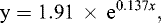 (2)
(2)
where y − salinity, g/l; x − age of the lake, years.
The comparison of equations for Lake Magic (Eq. (2)) and for the lower lake (Fig. 6) showed that salinity could grow approximately two times faster in Lake Magic than observed in the lower lake. The reasons for such differences should be inspected in more detail with future studies. Using equation (2), we calculated the possible salinity in Lake Magic in 2030 and 2040. These values are 61 g/l in 2030 and 240 g/l in 2040. Calculated salinity (Fig. 6) in the upper lake maybe 2.2 and 2.5 g/l, respectively in 2030 and 2040. Calculated salinity (Fig. 6) in the lower lake maybe 59 and 128 g/l, in 2030 and 2040, respectively. A salinity increase may lead to the formation of anoxic and hypoxic events near the bottom resulting in the ecosystem's changes and species richness reduction, similar to that in Lake Qarun (Shadrin et al., 2016). In the next five to six years, an occasional invasion of marine organisms is likely to continue in Lake Magic due to the release of fish fry into the lake as it was observed in Lake Qarun (El-Shabrawy et al., 2015; Shadrin et al., 2016). Later, a salinity increase will eliminate even these marine species.
Currently, Lake Magic is used only for tourism activities due to its marvel color variability. There is a plan to develop fishery and aquaculture in it as in other lakes of the depression. Mullet fry has been introduced into the lake at the end of 2019. Taking into account the halotolerance of mullet species (Anufriieva, 2018), it is predicted that the lake could support a small-scale mullet fishery for 10–12 years, but not more. Due to the fast growth of salinity, the fishery cannot be assumed as a perspective here. Only some hypersaline aquaculture can be developed as a long-term perspective, and most promising objects are brine shrimp and chironomid larvae (Anufriieva, 2018). Small lakes provide an opportunity to understand intra-ecosystem connectivity and its dynamics. We hope that these results can be used as the starting point for the long-time monitoring of changes in Lake Magic. This should provide an important contribution to our knowledge of arid area lakes' response to climate variability.
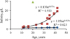 |
Fig. 6 Salinity changes in lakes of Wadi El Rayan depression (blue rhombuses − the upper lake, red squares − the lower lake, green triangles − Lake Magic). |
Conflicts of interest
The authors declare no conflict of interest.
Acknowledgments
Sampling and sample processing, data analysis, and manuscript writing were conducted in the framework of the state assignments of the National Institute of Oceanography and Fisheries (Egypt) and the A.O. Kovalevsky Institute of Biology of the Southern Seas of RAS (Russia) (№ АААА-А19-119100790153-3). The authors thank Prof. Jonathan Clark (USA) for his help to improve English.
References
- Afefe AA, Hatab EB, Abbas MS, Gaber ES. 2016. Assessment of threats to vegetation cover in Wadi El Rayan Protected Area, western desert, Egypt. Int J Conserv Sci 7: 691–708. [Google Scholar]
- Al-Yamani FY, Skryabin V, Gubanova A, Khvorov S, Prusova I. 2011. Marine zooplankton practical guide. Kuwait Institute for Scientific Research, Kuwait, 399 p. [Google Scholar]
- American Public Health Association (APHA). 2005. Standard methods for the examination of water and wastewater, 21st edition; American Public Health Association/American Water Works Association/Water Environment Federation, Washington D.C., USA. [Google Scholar]
- Anagnostidis K, Komárek J. 1988. Modern approach to the classification system of cyanophytes. 3. Oscillatoriales. Algolog Stud/Arch Hydrobiol 50–53: 327–472. [Google Scholar]
- Anufriieva EV. 2018. How can saline and hypersaline lakes contribute to aquaculture development. A review. J Oceanol Limnol 36: 2002–2009. [CrossRef] [Google Scholar]
- Black GF. 1988. Description of the Salton Sea sport fishery, 1982–1983; Inland Fisheries Administrative Report No. 88–89. California Department of Fish and Game, Long Beach, California, 50 p. [Google Scholar]
- Cohen MJ. 2009. Past and future of the Salton Sea. In Gleick PH, Cohen MJ, eds. The World's Water 2008–2009: The Biennial Report on Freshwater Resources. Washington, DC, USA: Island Press, pp. 133–147. [Google Scholar]
- Conway DVP. 2012. Marine zooplankton of southern Britain. Part 1: Radiolaria, Heliozoa, Foraminifera, Ciliophora, Cnidaria, Ctenophora, Platyhelminthes, Nemertea, Rotifera and Mollusca. Occasional Publications. Marine Biological Association of the United Kingdom, No. 25, Plymouth, United Kingdom, 138 p. [Google Scholar]
- Conway DVP. 2012. Marine zooplankton of southern Britain. Part 2: Arachnida, Pycnogonida, Cladocera, Facetotecta, Cirripedia and Copepoda. Occasional Publications. Marine Biological Association of the United Kingdom, No 26 Plymouth, United Kingdom 163 p. [Google Scholar]
- Downing JA. 2010. Emerging global role of small lakes and ponds: little things mean a lot. Limnetica 29: 9–24. [Google Scholar]
- Egypt today. Available online: https://www.egypttoday.com/Article/9/13788/Fayoum's-Magic-Lake ( accessed on Tuesday, July 25, 2017) [Google Scholar]
- Egyptian Environmental Affairs Agency (EEAA). 2017. Summary report of the environmental monitoring program for Egyptian lakes, El-Rayan lakes. Egyptian Environmental Affairs Agency, Ministry of Environment, Egypt. (In Arabic) http://www.eeaa.gov.eg/en-us/topics/water/lakes.aspx [Google Scholar]
- El Gammal EA, El Gammal AE. 2010. Human impact on landscape and the revenue in Wadi El Rayan Western Desert Egypt. Proceeding of the International Conference on Environmental Research and Technology (ICERT 2010), School of Industrial Technology, Universiti Sains Malaysia. [Google Scholar]
- El-Shabrawy GM, Anufriieva EV, Germoush MO, Goher ME, Shadrin NV. 2015. Does salinity change determine zooplankton variability in the saline Qarun Lake (Egypt). Chin J Oceanol Limnol 33: 1368–1377. [Google Scholar]
- El-Shabrawy GM, Dumont HJ. 2009. The Fayum depression and its lakes. In: Dumont HJ, ed. The Nile. Springer, Dordrecht, 95–124. [CrossRef] [Google Scholar]
- EL-Shabrawy GM, Hussian AM. 2015. Limnology, fauna and flora of Wadi El-Rayan Lakes and its adjacent area, Fayum, Egypt. In EL-Shabrawy G, Gopal B, Ghabbour S, eds. Limnology, Animals and Plants. Paris, France: Eolss Publishers, 1–10. [Google Scholar]
- Goher ME, Mahdy ES, Abdo MH, Farida M, Korium MA, Elsherif AA. 2019. Water quality status and pollution indices of Wadi El-Rayan lakes, El-Fayoum, Egypt. Sustain Water Resourc Manag 5: 387–400. [CrossRef] [Google Scholar]
- Hammer UT. 1986. Saline lake ecosystems of the world. Dordrecht, Netherlands: Dr. W. Junk Publishers, 616 p. [Google Scholar]
- Han MW, Park YC. 1999. The development of anoxia in the artificial Lake Shihwa, Korea, as a consequence of intertidal reclamation. Mar Pollut Bull 38: 1194–1199. [Google Scholar]
- Hassan FA. 1986. Holocene lakes and prehistoric settlements of the western Fayum, Egypt. J Archaeolog Sci 13: 483–501. [CrossRef] [Google Scholar]
- Hely AG, Hughes GH, Irelan B. 1966. Hydrologic regimen of Salton Sea, California. United States Geological Survey Professional Paper 486-C. United States Government Printing Office, Washington, 32 p. [Google Scholar]
- Huber-Pestalozzi G. 1961. The freshwater phytoplankton. Taxonomy and biology. 5. Chlorophyceae (green algae), the order Volvocales. In: Thienemann A, ed. Inland waters. E. Schweizerbart'sche Verlasbuchhandlung, Stuttgart, Vol. 3, 744 p. (In German). [Google Scholar]
- Huber-Pestalozzi G. 1983. The freshwater phytoplankton. Taxonomy and biology. 7(1). Chlorophyceae (green algae), the order Chlorococcales. In: Thienemann A, ed. Inland waters. E. Schweizerbart'sche Verlasbuchhandlung, Stuttgart, Vol. 16, 1044 p. (In German). [Google Scholar]
- Hussein H, Amer R, Gaballah A, Refaat Y, Abdel-Wahab A. 2008. Pollution monitoring for Lake Qarun. Adv Environ Biol 2: 70–80. [Google Scholar]
- Komárek J, Anagnostidis K. 1999. Cyanoprokaryota.1. Chroococcales. In Ettl H, Gerlo J, Heynig H, Mollenhauer D, eds. The freshwater flora of Central Europe. Gustaw Fischer, Jena, 1–548. (In German). [Google Scholar]
- Komárek J, Anagnostidis K. 1986. Modern approach to the classification system of cyanophytes. 2. Chroococcales. Algolog Stud/Arch Hydrobiolog 43: 157–226. [Google Scholar]
- Komárek J, Anagnostidis K. 1989. Modern approach to the classification system of cyanophytes. 4. Nostocales. Algolog Stud/Arch Hydrobiolog 56: 247–345. [Google Scholar]
- Krammer K, Lange-Bertalot H. 1986. Bacillariophyceae. 1. Naviculaceae. In: Pascher A, ed. The freshwater flora of Central Europe. Gustaw Fischer, Jena, 1–876. (In German). [Google Scholar]
- Krammer K, Lange-Bertalot H. 1988. Bacillariophyceae. 2. Epithemiaceae, Surirellaceae. In: Pascher A, ed. The freshwater flora of Central Europe. Gustaw Fischer, New York, 1–596. (In German). [Google Scholar]
- Krammer K, Lange-Bertalot H. 1991a. Bacillariophyceae. 3. Centrales, Fragilariaceae, Eunotiaceae. In: Pascher A, ed. The freshwater flora of Central Europe. Gustaw Fischer, Jena, 1–576. (In German). [Google Scholar]
- Krammer K, Lange-Bertalot H. 1991b. Bacillariophyceae. 4. Achnanthaceae, critical supplement to Navicula (Lineolatae) and Gomphonema. In: Pascher A, ed. The freshwater flora of Central Europe. Gustaw Fischer, Jena, 1–433. (In German). [Google Scholar]
- Kurlansky M. 2002. Salt: a world history. Penguin, New York, USA, 496 p. [Google Scholar]
- Maiyza IA, El-Rhaman MA, Ellah RA. 1999. Evaporation from Wadi El Rayan lakes, Egypt. Bull Natl Inst Oceanogr Fish 25: 79–88. [Google Scholar]
- Mansour SA, Sidky MM. 2003. Ecotoxicological Studies. 6. The first comparative study between Lake Qarun and Wadi El-Rayan wetland (Egypt), with respect to contamination of their major components. Food Chem 82: 181–189. [Google Scholar]
- Mohamed FAS, Sabae SZ. 2015. Monitoring of pollution in Wadi El-Rayan lakes and its impact on fish. Int J Dev 4: 1–28. [CrossRef] [Google Scholar]
- Müller PH, Neuman P, Storm R. 1979. Tafeln der Mathematischen Statistik. VEB Fachbuchverlag Leipzig, Germany, 272 p. [Google Scholar]
- Popovský I, Pfiester LA. 1990. Dinophyceae (Dinoflagellida). In Ettl H, Gerlo J, Heynig H, Mollenhauer D, eds. The freshwater flora of Central Europe. Gustaw Fischer, Jena, 1–272. (In German). [Google Scholar]
- Ramzy YH. 2013. Sustainable tourism development in Al Fayoum Oasis, Egypt. WIT Trans Ecol Environ 175: 161–173. [CrossRef] [Google Scholar]
- Rudescu L. 1960. Fauna Republicii Populare Romine, Trochelminthes (Rotatoria), Volumul II. Fascicula II. Editura Academiei R. P. R., Bucuresti, 1192 p. [Google Scholar]
- Sayed MF, Abdel-Satar AM. 2009. Chemical assessment of Wadi El-Rayan Lakes-Egypt. Am-Euras J Agric Environ Sci 5: 53–62. [CrossRef] [Google Scholar]
- Schroeder RA, Orem WH, Kharaka YK. 2002. Chemical evolution of the Salton Sea, California: nutrient and selenium dynamics. In Barnum DA, Elder JF, Stephens D, Friend M, eds. The Salton Sea. Springer, Dordrecht, 23–45. [CrossRef] [Google Scholar]
- Shadrin N, Anufriieva E, Galagovets E. 2012. Distribution and historical biogeography of Artemia Leach, 1819 (Crustacea: Anostraca) in Ukraine. Int J Artemia Biol 2: 30–42. [Google Scholar]
- Shadrin NV, El-Shabrawy GM, Anufriieva EV, Goher ME, Ragab E. 2016. Long-term changes of physicochemical parameters and benthos in Lake Qarun (Egypt): Can we make a correct forecast of ecosystem future. Knowl Manag Aquat Ecosyst 417: 18. [CrossRef] [Google Scholar]
- Shalloof KA. 2020. State of fisheries in Lake Qarun, Egypt. J Egypt Acad Soc Environ Dev D Environ Stud 21: 1–10. [CrossRef] [Google Scholar]
- Shuford WD, Warnock N, Molina KC, Sturm KK. 2002. The Salton Sea as critical habitat to migratory and resident waterbirds. Hydrobiologia 473: 255–274. [Google Scholar]
- Sokal RR, Rohlf FJ. 1995. Biometry: The principles and practice in biological research. New York: Freeman, 880 p. [Google Scholar]
- Thode HC. 2002. Testing for normality. New York: Marcel Dekker Inc., 479 p. [Google Scholar]
- Vilenica M, Pozojević I, Vučković N, Mihaljević Z. 2020. How suitable are man-made water bodies as habitats for Odonata. Knowl Manag Aquat Ecosyst 421: 13. [CrossRef] [Google Scholar]
- Voyles TB. 2016. Environmentalism in the interstices: California's Salton Sea and the borderlands of nature and culture. Resilience 3: 211–241. [Google Scholar]
- World Health Organization (WHO). 2001. Water Quality: Guidelines, Standards and Health. London, UK: IWA Publishing, 413 p. [Google Scholar]
- Yamaji I. 1978. Illistrations of the marine plankton of Japan. Osaka: Hoikush Publishing Co., 483 p. [Google Scholar]
Cite this article as: Anufriieva EV, Goher ME, Hussian AEM, El-Sayed SM, Hegab MH, Tahoun UM, Shadrin NV. 2020. Ecosystems of artificial saline lakes. A case of Lake Magic in Wadi El-Rayan depression (Egypt). Knowl. Manag. Aquat. Ecosyst., 421, 31.
All Tables
Coordinates and some characteristics of sampling sites in Magic Lake during January 2019.
Correlations between different chemical characteristics of water in Magic Lake during January 2019.
All Figures
|
Fig. 1 Lake Magic location and distribution of the sampling sites. |
| In the text | |
|
Fig. 2 Similarities between the sampling sites according different abiotic characteristics (a − clustering of sites according chemical characteristics from Tabs. 2 and 3; b − clustering of sites according heavy metals content characteristics from Tab. 4). |
| In the text | |
|
Fig. 3 Clustering of sites according phytoplankton (a), microbiological characteristics (b), zooplankton (c). |
| In the text | |
|
Fig. 4 Phytoplankton in Magic Lake during January 2019 (a − chlorophyll a distribution, b − correlation between chlorophyll a content and phytoplankton abundance). |
| In the text | |
|
Fig. 5 Distribution of bacterial indicators in Lake Magic during January 2019 (1–TVBC at 37 °C, 102 CFU/m; 2–TVBC at 22 °C, 102 CFU/m; 3–TC, MPN/100 ml; 4–FC, MPN/100 ml; 5–FS, 102 MPN/100 ml). |
| In the text | |
|
Fig. 6 Salinity changes in lakes of Wadi El Rayan depression (blue rhombuses − the upper lake, red squares − the lower lake, green triangles − Lake Magic). |
| In the text | |
Current usage metrics show cumulative count of Article Views (full-text article views including HTML views, PDF and ePub downloads, according to the available data) and Abstracts Views on Vision4Press platform.
Data correspond to usage on the plateform after 2015. The current usage metrics is available 48-96 hours after online publication and is updated daily on week days.
Initial download of the metrics may take a while.