| Issue |
Knowl. Manag. Aquat. Ecosyst.
Number 426, 2025
Riparian ecology and management
|
|
|---|---|---|
| Article Number | 21 | |
| Number of page(s) | 11 | |
| DOI | https://doi.org/10.1051/kmae/2025016 | |
| Published online | 17 July 2025 | |
Research Paper
Monitoring the impact of small hydroelectric plants in the Alps: an interesting case study from NW Italy
1
DBIOS, University of Turin, Via Accademia Albertina, 13, 10123 Turin, Italy
2
ALPSTREAM – Alpine Stream Research Center, Parco del Monviso, 12030 Ostana, Italy
3
Freelance Ichthyologist - NATURASTAFF - Via del Ricetto, 6, 15077 Predosa, Italy
* Corresponding author: This email address is being protected from spambots. You need JavaScript enabled to view it.
Received:
24
February
2025
Accepted:
16
June
2025
Abstract
Alpine streams are valuable ecosystems for biodiversity and ecological function but are highly vulnerable to global and local stressors. Climate change represents a major global threat, while the growing development of small hydropower plants (SHPs) poses a significant risk to the integrity of Alpine lotic systems. This study examined the construction and implementation of an SHP in the Cottian Alps (NW Italy), assessing environmental quality and biodiversity indicators (macroinvertebrates and fish) over time. The STAR_ICMi index (standardised) and the FlowT index (innovative) were applied to evaluate SHP impact but revealed no differences: the ecological status was consistently rated as “good”, and no post-operam changes related to flow alterations were observed among the three stations (S1 = upstream, S2 = tail, S3 = downstream) when analysing macroinvertebrate rheophilia. Environmental parameters measured also showed no significant variation over time. However, some biological parameters did reveal changes. Macroinvertebrate abundance was significantly lower at S2, while taxa richness differed between the ante-operam and post-operam phases. Functional feeding groups remained unchanged. For fish, total abundance increased, though density and biomass stayed stable. Although the indices retained suggest minimal impact, the study underscores the need to integrate specific biological parameters into monitoring programmes for a more precise ecological assessment.
Key words: macroinvertebrates / fish communities / hydropower / lotic systems / environmental monitoring
© M. Moriondo et al., Published by EDP Sciences 2025
 This is an Open Access article distributed under the terms of the Creative Commons Attribution License CC-BY-ND (https://creativecommons.org/licenses/by-nd/4.0/), which permits unrestricted use, distribution, and reproduction in any medium, provided the original work is properly cited. If you remix, transform, or build upon the material, you may not distribute the modified material.
1 Introduction
Alpine ecosystems, in the strict sense of the term, are peculiar environments found between the treeline and the permanent snowline (Brown et al., 2015), and they are represented across all continents and latitudes (Körner, 2003; Testolin et al., 2020). Water is generally abundant in these environments (Pomeroy et al., 2015) and can come from a variety of sources: glacial and rock glacier meltwater, snowmelt, and groundwater (Milner and Petts, 1994; Ward, 1994; Malard et al., 1999; Füreder et al., 2001; Brighenti et al., 2019), resulting in a considerable heterogeneity of freshwater habitats and biodiversity (Füreder, 1999; Brown et al., 2003).
Alpine streams, despite their different origins, share some characteristics such as high slope, high water flow velocity, high dissolved oxygen concentrations, low water temperature, and reduced trophic status (Milner and Petts, 1994; Ward, 1994; Tockner et al., 2002), which combine to make these streams a harsh and selective environment (Füreder et al., 2001). As a result, the animal and plant communities that live there consist of specialised organisms well adapted to these extreme conditions (Füreder, 1999). Being specialised, however, also means being vulnerable to change. Despite their remoteness, Alpine streams are now exposed to a range of hydrological and chemical stressors.
Regarding hydrological stressors, one of the most important is the alteration of streamflow due to hydropower production (Chiogna et al., 2016), which is the largest used source of renewable energy globally (Wasti et al., 2022). Although hydropower does not actually consume water, it can affect the integrity of river ecosystems at several levels. For instance, hydropower plant alters the waterflow converting river reaches into reservoirs and causing short-term (hydropeaking) or seasonal changes in the flow regime; interrupts sediment transport, degrading floodplain habitats downstream of dams; often creates insurmountable barriers for lotic organisms that could lead to genetic isolation; alters the thermal regime by releasing hypolimnetic water from reservoirs; affects water quality through phytoplankton growth in reservoirs potentially leading to a shift from heterotrophy to autotrophy (e.g., Olden and Naiman, 2010; Viviroli et al., 2011; Guareschi et al., 2014; Costea et al., 2021; He et al., 2024).
Large hydropower systems have received more attention than small hydropower plants (SHP) (Jager et al., 2015; Lin et al., 2024), which, however, account for about 90% of hydropower facilities globally (Couto and Olden, 2018). SHPs have been shown to produce a relatively modest amount of electricity, yet they have become increasingly prevalent in recent decades, with a notable presence in a wide variety of streams and creeks, including those of a relatively modest size (Couto and Olden, 2018; Lin et al., 2024). SHP usually refers to plants with an installed capacity of less than 10 MW (Lange et al., 2019). Some authors have highlighted how, despite their small size, SHPs have a dramatic impact on running water ecosystems and in particular on their biodiversity (Xiaocheng et al., 2008; Kibler and Tullos, 2013; Couto et al., 2023).
Macroinvertebrate communities play a crucial role in the function and dynamics of river ecosystems due to their involvement in numerous processes such as biomass production, nutrient cycling and resource processing (Merrit et al., 1984). Benthic macroinvertebrates are the most widely used group of organisms in freshwater biomonitoring (Resh, 2008; Dagnino et al., 2013) due to their sensitivity to changes in both water chemistry and habitat physical properties (Bo et al., 2006; Rossaro et al., 2011; Buss et al., 2015). Furthermore, they are abundant, easy to collect and have a relatively long-life cycle, making the analysis of their community structure an effective tool for detecting human pressures and stressors over long periods of time (Buss et al., 2015; Bolpagni et al., 2017). As macroinvertebrates are strongly influenced by hydro-morphological conditions and flow alterations, they have long been included in impact assessment studies for hydropower plants and dams, including SHPs (e.g. Guareschi et al., 2014; González et al., 2018; Krajenbrink et al., 2019; Laini et al., 2019; Lin et al., 2024). In these contexts, the most critical areas for the macroinvertebrate community are essentially the dam-induced reservoirs and the sections drained downstream. In these areas, standing water species can replace those typically present under flowing conditions, with lower values of diversity indices compared to other sites, with filterers and collectors dominating the functional feeding groups (e.g. Merritt et al., 2017; Lin et al., 2024). Another biotic component affected by alterations in streamflow is freshwater fish, one of the most threatened groups due to the numerous pressures on freshwater environments (Dudgeon et al., 2006; Freyhof and Brooks, 2011; Dudgeon, 2019; Abbà et al., 2024). These include environmental changes caused by dams and hydropower plants, the effects of which have been documented in several studies (e.g. Cooper et al., 2017; Costea et al., 2021). In particular, changes in both fish abundance and community have been observed, with rheophilic and specialised species being replaced by more generalised species adapted to lentic habitats (Cooper et al., 2017; Costea et al., 2021). Similar effects were found in studies of the impacts of SHPs, which showed a reduction in density, biomass and total abundance at impacted sites (Kubečka et al., 1997; Almodovar and Nicola, 1999; Benejam et al., 2016), as well as lower values of some parameters such as mean fork length, total weight, and fish health status (Benejam et al., 2016). A study focusing on an indigenous population of brown trout showed a loss of small and juvenile individuals as a consequence of SHP (Almodovar and Nicola, 1999). Other studies of multi-species communities have shown a decrease in large-sized species and an increase in small, lentic-adapted species (e.g., Kubečka et al., 1997; Couto et al., 2023). Underlying these impacts is the depletion of stream habitat quality caused by these facilities, which results in fewer fish refuges and altered water depth (Benejam et al., 2016), as well as the presence of barriers that can prevent upstream migration (Anderson et al., 2006).
The potential impacts of SHPs can be attributed to the characteristics of the ecosystem involved and the type of facility. Indeed, SHPs with the same installed capacity may have significantly different dam sizes, reservoir areas, storage capacities, outlet structures, and operational procedures (Couto and Olden, 2018). Currently, most of the available studies concern temperate and tropical ecosystems (Anderson et al., 2006; Arantes et al., 2019), while other environments, such as alpine, remain less investigated.
In this research, we evaluated the impact of a SHP in the north-western Italian Alps.
The objectives of this study were: i) to describe the physico-chemical profile of the area; ii) to investigate the response of macroinvertebrate and fish communities to the implementation of the SHP and iii) to test the performance of a traditional index used in biomonitoring to assess the ecological status, STAR_ICMi, with an unconventional one, FlowT (Laini et al., 2022a). The study utilised a six-year time series of data, encompassing the period preceding, during, and following the construction of the small hydroelectric plant.
2 Materials and methods
2.1 Study area
Ripa River is a right tributary of the Dora Riparia stream (Italian Cottian Alps − Fig. 1a). This lotic system is 25 km long and rises in the municipality of Sauze di Cesana (TO) between the “Cima Roudel” (2,994 m a.s.l.) and the “Punta della Scodella” (2,895 m a.s.l.) and flows into the homonymous valley (also known as Argentera Valley).
The studied area is characterized by the presence of extensive mountain woods consisting mainly of native conifers (e.g. Larix decidua Miller, 1768, Pinus cembra Linneo, 1753, Abies alba Miller, 1759). Ripa stream flows in a wide channel characterized by an elevated slope (15.97% in the studied stretch) and substrate dominated by boulders, cobbles and gravels. The climate is temperate-alpine, with summertime high discharge caused by snowmelt.
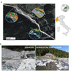 |
Fig. 1 a. Study area, details of the stations displayed: S1 = up, S2 = tail and S3 = down. b. Photos: on the left derivation and associated fish ladder, on the right the hydroelectric power station externally. |
2.2 Hydroelectric plant
From 2017 to 2018, a new hydroelectric power plant was built with a maximum derived discharge of 2,400 L/sec and a medium annual value of 825 L/sec. The derivation is made of a cement barrier, with water intake by falling through a grid and an artificial passage for fish fauna on the left bank (Fig. 1b).
Sampling areas were selected along a river stretch of 1.9 km length and three stretches were sampled from November 2016 to February 2022. In total, 11 monitoring campaigns were conducted, distributed as reported in Table 1. The stations were designated as follows: “S1” (N 44°55'31,7” − E 6°52'36,2” 1,650 m a.s.l.), upstream of the diversion for hydroelectric use, “S2” (N 44°56'03,3” − E 6°51'58,7”; 1,560 m a.s.l.), at the tail, i.e. in the section subtended by the plant and “S3” (N 44°56'14,7” − E 6°51'46,2”; 1,535 m a.s.l.), downstream of the restitution (Fig. 1a). Before the realization of this studied hydroelectric plant, we carried out a monitoring campaign (November 2016) hereinafter referred to as “Ante Operam − A.O.”. During the construction of the hydroelectric infrastructure, we carried out a second monitoring campaign, named “Construction phase − C.P.” (September 2017). Following the end of the plant construction, we have carried out nine monitoring campaigns during the productive phase, denominated “Post Operam − P.O.” (from January 2019 to February 2022).
During the monitoring campaigns we collected i) surface water samples for the assessment of main chemical and bacteriological parameters and ii) quantitative samples of macroinvertebrates and fish to evaluate community composition and structure.
Frequency of samplings and investigated indicators.
2.3 Chemical and physical analysis
During the study period, water and air temperatures were measured using a field thermometer (ThermoPro model TP01S), while in the laboratory mainly physical-chemical and bacteriological parameters were measured after surface water sampling (Tab. 2).
Main physical and chemical parameters measured during the study period.
2.4 Macroinvertebrates sampling and processing
In the three sections of the examined stream, an estimation of depths and substrate composition of the riverbed was carried out, noting the degree of coverage of mineral components (mud, sand, gravel, stones of various size classes) and biotic components (such as fallen leaves, mosses, macrophytes and dead wood). It was then determined at which points to take ten quantitative Surber samples, weighted according to the frequency of substrate categories in the water body, thus applying multi-habitat sampling (Buffagni et al., 2008; IRSA 2008 and 2014). Quantitative samples of benthic macroinvertebrates were collected using a Surber sampler (25 × 25 cm, mesh = 255 μm) and were sorted in the field as requested by the legislation. A total of 330 Surber samples were collected, equally distributed across the three sampling sites. A preliminary analysis of the data obtained by plotting taxa accumulation curves showed that the sampling effort was largely adequate to obtain a representative characterization of the diversity of macroinvertebrate communities at the sites.
Subsequently, macroinvertebrates were counted and systematically identified in laboratory at the family or genus level, according to the Italian dichotomous key for benthic macroinvertebrate fauna (Campaioli et al., 1994; Campaioli et al., 1999; Messori, 2006; Fochetti and Tierno de Figueroa 2008; Tachet et al., 2010). The total number of taxa and the total number of individuals were then calculated for each sample. With these data we calculated the STAR_ICMi index according to current Italian legislation. This biotic index is the official tool used for the evaluation of biological quality of Italian lotic systems (Buffagni et al., 2008).
2.5 Fish sampling and processing
In the three studied stream sections we also collected fish fauna. Fish were caught along a 100 m transect, using a Scubla ELT 60 II GI electro-fishing device. Total sampled area has been calculated by measuring the average width of the wet riverbed multiplied by the length of the monitored stretch. In this way it is possible to get the number of individuals/m2 and total biomass (g/m2).
After two passes, all collected fish were identified at the species level, measured and weighed individually. Before handling, they were anaesthetized with a non-invasive solution of cloves and ethanol (1:9). After measurement all the specimens were placed in a fish-cage waiting to be released into the stream.
2.6 Statistical analyses
Variance inflation factor (VIF) analysis was applied to the annual means calculated for the measured physico-chemical water parameters, using the usdm R package (Naimi et al., 2014) to exclude variables with the highest multicollinearity (VIF > 2).
For the remaining six water quality variables (Escherichia coli, conductivity, ammonia nitrogen, COD, total phosphorus and dissolved oxygen) linear mixed effects models (LMM) were performed using the lmerTest R package (LMM, Kuznetsova et al., 2017), to test whether there were differences between the three phases (A.O., C.P. and P.O.) considering the “monitoring station”, i.e. S1, S2, S3, and “year” as random factors. In the case of the ammonia nitrogen parameter, there were no “monitoring stations” related effects, so we opted to simplify the model by including only “year” as a random factor. LMMs were also applied to macroinvertebrate and fish community data. For the macrobenthos, the total abundance and taxonomic richness of taxa, the abundance and taxonomic richness of Ephemeroptera, Plecoptera and Trichoptera (EPT), and the percentage dominance of the first three taxa (DOM-3) between stations, years and phases were analysed, each time considering two of these factors as random. The model was simplified with a single random factor when the second one had no influence, keeping the version with the lowest AIC (Sakamoto et al., 1986). Furthermore, potential differences in functional community metrics regarding feeding functional groups (FFGs) were examined. The relative abundances of the 5 FFGs per station over the 6 years were calculated and described. Linear mixed models were used to test whether there were differences between the monitored stations, considering both “year” and “phase” as random factors when they had effects or otherwise removing them to simplify the model by selecting the lowest AIC value.
The FlowT index (Laini et al., 2022a) was applied to macroinvertebrate presence-absence data to assess the effects of flow regime changes on macroinvertebrate communities across the three monitored areas in the P.O. phase. This index quantifies rheophilic preferences and was calculated using the R package biomonitoR (Laini et al., 2022b). A linear mixed effects model was used to determine the variation between S1, S2 and S3, with “year” as a random factor.
For fish communities, the LMM test was used to detect differences in total abundance, total taxa richness, density (N/m2) and biomass (g/m2) between stations, years and phases, each time considering the two non-independent variables as random factors when influent or using a simplified model if not. Model hypotheses were tested graphically using the predictmeans R package (Luo et al., 2024), and when necessary, pairwise comparisons were conducted with the emmeans R package (Lenth, 2024). All analyses were performed in the R statistical environment (R Core Team 2020), using the ggplot2 (Wickham, 2011) and ggalluvial (Brunson, 2020) packages for graphical representation. The significance threshold was set at p < 0.05.
3 Results
3.1 Physical-chemical parameters
The results of the mean values of water and air temperature and of the main chemical parameters measured at the different stations (S1, S2, S3) during each year of the study period are shown in Table (SM1).
To obtain a more detailed overview, comparisons were made of the physico-chemical parameters recorded over the six years in the three construction phases for the six variables that did not present problems of collinearity. The results are shown in Figure 2. The LMM test showed that there is no significant difference over time (p-value > 0.05) for any of the environmental parameters analysed.
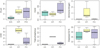 |
Fig. 2 Boxplots for the six chemical-physical parameters: E. coli = Escherichia coli (cfu), Cond = Conductivity (μS/cm), Ammonia nitrogen = Ammonia nitrogen (mg/L), COD = COD (mg/L), Total phosphorous = Total phosphorus (mg/L), Dissolved O2% = Dissolved Oxigen (% saturation); analysed in the three monitoring phases (A.O., C.P., P.O.). Median values are represented by a horizontal bold line. A.O. = 3obs., C.P. = 3obs. and P.O. = 12obs. |
3.2 Macroinvertebrates and STAR_ICMi Biotic Index
In total we collected 18,706 freshwater invertebrates belonging to 33 families. The most abundant taxa in the studied river stretch were: Leuctridae (Plecoptera) (33.86% of total), Chironomidae (Diptera) (16.45%) and Baetidae (Ephemeroptera) (16.03%) (Fig. 3).
The macroinvertebrates abundance (N) showed a statistically significant difference among the three stations (Fig. 4) (p-value = 0.0004, F value = 10.36).
Pairwise comparison shows that S2 has significantly lower values than S3 (S3vsS2: estimate = 285.5, p-value = 0.0004) and S1 (S2vsS1: estimate = -213.9, p-value = 0.0076). In contrast, there was no significant difference in the different years (p-value = 0.41, F value = 1.47) and phases (p-value = 0.17, F value = 1.92) (Fig. 5). This suggests that the abundance of macroinvertebrates is relatively stable over time and not particularly influenced by seasonal or inter-annual conditions.
Taxa richness (S) shows a different pattern (Fig. 5) with a significant variation between phases (p-value = 0.002, F value = 7,64), from the pairwise comparison there is a significant difference between A.O. and P.O., (estimate = 3.74, p-value = 0.002).
However, there was no significant difference between stations (p-value = 0.66, F value = 0.43) and year (p-value = 0.16, F value = 3.36) (Fig. 4). This indicates that the diversity between stations is fairly uniform.
The abundance of the EPT taxa (Fig. 6) varied significantly between stations (p-value = 0.015, F value = 4.89), from the pairwise comparison there is a significant difference between S3 and S2, (estimate = 215.6, p-value = 0.0129). These results suggest that local factors have an important influence on the abundance of these sensitive taxa. While there is no significant effect between years (p-value = 0.59, F value = 0.32) and between phases (p-value = 0.07, F value = 2.88), indicating that there was no consistent variation over time. Instead, the specific richness of EPT taxa did not vary significantly between stations and years, p-values > 0.05 were obtained for both, but there is a significant difference for the phases (p-value = 0.03, F value = 4.12) and from the pairwise comparison there is a significant difference between A.O. and P.O. (estimate = 2, p-value = 0.0209).
The dominant taxa (DOM-3) showed significant variation between phases (p-value = 0.025, F value = 9.56), the pairwise comparisons show there is a significant difference between C.P. and P.O. (estimate = −28.3, p-value = 0.0263). While there is no significant difference for stations and years both have a p-value > 0.05.
Regarding the functional feedings groups (FFGs) in terms of percentages per station over the years (Fig. 7), the highest value obtained is that of the shredders, which was 56.73% in S1 in 2022, followed by the predators with 56.18% in station S3 in 2017. In third place are the collectors with 53.42% in S2 in 2022, while lower numbers are found for the scrapers, with a maximum value of 12.05% obtained in S2 in 2016, and for the filter feeders, which recorded a maximum of 1.34% in S1 in 2020. The LMM test showed no significant differences for the 5 (FFG) between the monitoring stations, p-value > 0.05.
In all the monitoring carried out, the river was in the “good” range of the STAR_ICMi biotic index.
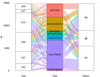 |
Fig. 3 Sankey diagram of the most abundant occurring taxa. On the y-axis are the cumulative abundances of the different taxa, on the x-axis are the distributions of the different taxa at the different monitoring sites in different years. Sankey diagrams of the remaining taxa are available in supplementary material Figure SM2. |
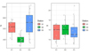 |
Fig. 4 Box plots showing macroinvertebrate abundance (N) and macroinvertebrate taxa richness (S) in the different monitoring stations: in salmon S1, in green S2 and in blue S3, 11 observations each, represented by the grey dots. Median values are represented by a horizontal bold line. |
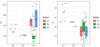 |
Fig. 5 Box plots showing macroinvertebrate abundance (N) and macroinvertebrate taxa richness (S) in the three different phases: in salmon S1, in green S2 and in blue S3, 11 observations each, represented by the dots. Median values are represented by a horizontal bold line. |
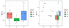 |
Fig 6 Box plots showing EPT abundance (N) and EPT richness (S) in the three monitoring stations and the three different phases: in salmon S1, in green S2 and in blue S3. Median values are represented by a horizontal bold line, the points represent 11 observations for each station and for each phase: A.O. = 3obs, C.P. = 3obs and P.O. = 9obs. |
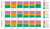 |
Fig. 7 Stacked bar charts of percentage frequencies of the five functional feeding groups (FFG) on the y-axis, in the different monitoring stations (S1, S2, S3) during the six years indicate on the x-axis. |
3.3 FlowT index
The value of the FlowT index calculated on the Post Operam (P.O.) monitoring data from the years 2019 to 2022 found no significant variations (p-values > 0.05, Fig. 8) in the three stations considered: upstream (S1), at tail of the plant (S2) and downstream (S3).
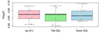 |
Fig. 8 Box plot showing the value of the FlowT index calculated post operam (P.O.) for the monitoring area: upstream (S1), at the tail (S2) and downstream (S3), 9 observations each station. Median values are represented by a horizontal bold line. |
3.4 Fish parameters
In total we collected 627 fish belonging to only one family: Salmonidae. In particular the collected specimens belonged to two species, the Brown trout (Salmo trutta, Linneo, 1758), n = 57, and the Mediterranean brown trout (Salmo ghigii, Pomini, 1941), n = 570. Mediterranean brown trout dominate the fish community, making up 90.9% of the total. Significant differences were found through LMM test for abundance (N) between years (p-value = 0.009, F value = 11.94), which has increased (Fig. 9) and for richness (S) between stations (Fig. SM3), with station S1 having a significantly different richness distribution (p-value < 0.05) from S2 and S3. No significant differences instead emerged for density and biomass between years, stations or phases.
 |
Fig. 9 Abundance (N), density(n/m2), biomass (g/m2) and richness (S) of fish in each different year campaign: red 2016, green 2019, blue 2020, yellow 2021. |
4 Discussion
A thorough examination of the data collected reveals that the environmental impact of the hydroelectric power plant is negligible. The chemical-physical parameters exhibited stability across the three phases that were monitored. Regarding macroinvertebrates, significant differences in community abundance were observed between the stations. In particular, the section that was subject to water extraction (station S2) exhibited the most disturbance, demonstrating significantly lower abundance values compared to the other two stations. Indeed, S2 generally showed lower values than the upstream station S1, a pattern that became more pronounced in the years following the SHP implementation. No significant differences were found between the three different phases. Significant differences emerged in richness (S) between the phases when considering the total community and the most sensitive EPT taxa, particularly between the A.O. and P.O. phases, with higher values recorded before the installation of the SHP. Regarding the dominant taxa (DOM-3), a significant difference was found between the C.P. and P.O. phases, with the construction phase showing lower values. This pattern corresponds probably to disturbances related to construction activities, which were no longer observed afterwards. Richness EPT and DOM-3 were not significant between the three different stations.
Focusing on the functional feeding groups (FFGs), no differences were found between the stations. In this respect, we can conclude that the assemblage was stable and equally diversified. Contrary to other studies (e.g., Merritt et al., 2017; Lin et al., 2024), we did not observe homogenisation; instead, collectors, predators, and shredders were consistently present at both S2 and S3. The same results were performed by STAR_ICMi index, which remained “good” throughout the monitoring period. The STAR_ICMi index is a widely used tool for assessing the biological status of water bodies, and its stability over the different sites indicates that the operation of the hydroelectric plant has not had a detrimental effect on the overall water quality and biological integrity of the Ripa stream. This suggests that the hydroelectric plant has not substantially alter the physical habitat or water quality in the Ripa stream (Česonienė et al., 2021). The FlowT index, whose function is to monitor the effect of flow variation, did not show any differences between the three monitoring stations (S1, S2, and S3) after the hydropower plant was started up. Its values remain stable and are characteristic of lotic environments influenced by an elevated discharge, such as rapids and riffles, (Laini et al., 2022a), which are typical of a mountain stream.
Similarly, the fish community was dominated by native salmonid species, suggesting that the environment resulted in a pristine status. Significant differences were found for abundance (N) over time, which increased especially in 2020 and 2021, and for richness (S) between the three stations where S1 had the lowest values. This is because the Brown trout was only found in S1 in 2020. For the other monitored fish parameters: density and biomass, no differences were observed between stations, years and phases. This shows that the hydroelectric plant's operations did not appear to significantly harm the fish populations or their environment. It also suggests that they probably also benefit from the presence of the fish ladder.
The index results showed that the construction of the small hydroelectric plant on the Ripa torrent did not have a significant impact on the aquatic ecosystem and its biological components, very similar to what was reported in this other study carried out in the Italian Central-Eastern Alps by Scotti et al., 2022.
However, a more detailed analysis revealed some local variations, particularly at the intermediate station (S2), where a decline in the abundance of macroinvertebrates was observed. Furthermore, a temporal variation in taxa richness was detected between the A.O. and P.O. phases of monitoring. These dynamics, not intercepted by the indices, highlight the importance of including specific parameters in the monitoring.
A thorough analysis was conducted on other indicators, including the composition of the functional groups for macroinvertebrates and for ichthyofauna, density and biomass. These indicators did not reveal any critical issues, indicating a robust resilience of the system. The plant has been designed on the basis of hydrological and ecological analyses with the aim of minimising impacts; this necessitates careful and seasonally modulated management in order to avoid excessive withdrawals. To ensure the sustainability of these interventions, it is imperative that current regulations are adhered to and that technical-environmental planning is conducted with precision (Couto and Olden, 2018; Kuriqi et al., 2021).
It is important to recognise that this study analysed a limited number of samples and that it was not possible to obtain detailed information on the different environmental aspects for ante-operam (A.O.) and post-operam (P.O.) comparisons. However, we believe that the study can be of some practical use, as it contributes to the knowledge of a phenomenon (the increase of small hydropower in the Alps) that has been of enormous importance in recent years. Furthermore, the data presented, although coming from a single case and being the result of monitoring activities, can be compared with similar situations and also be processed and shared with the scientific community to increase knowledge on these issues that are of relevant interest.
Acknowledgments
We would like to thank Candiotto L., Guafa E. for their help during sampling activities and Bazzano F. for providing the data collected as part of the verification of his hydroelectric plant. The authors wish to thank Guareschi S. for providing valuable advice that greatly improved the manuscript. Marta Moriondo was supported by an INPS scholarship bound to research topics n.5 (field: Sustainable Development), project title “New indicators for the sustainable use of water resources and biodiversity conservation in Alpine rivers”.
Author contributions
TB and SF conceived the idea and designed the methodology; TB, AC provided the raw data; AM and MM analysed the data; MM, MA, AM lead the writing and composed the manuscript. All authors read and approved the final manuscript.
Disclosure statement
The authors have no conflicts of interest to report.
Supplementary Material
Table SM1. Mean values of environmental and chemical parameters measured during the study period, details of stations S1=up, S2=tail, S3=down.
Fig. SM2. Sankey diagram of the remaining macroinvertebrate taxa present. On the y-axis are the cumulative abundances of the different taxa, on the x-axis are the distributions of the different taxa at the different monitoring sites in different years.
Fig. SM3. Box plots showing fish richness (S) in the three different monitoring stations: S1 (up), S2 (tail) and S3 (down). There are four observations each station, represented by the dots and median values are represented by a horizontal bold line.
Access Supplementary MaterialReferences
- Abbà M, Ruffino C, Bo T, Bonetto D, Bovero S, Candiotto A, Comoglio C, Lo Conte P, Nyqvist D, Spairani M, Fenoglio S. 2024. Distribution of fish species in the upper Po River Basin (NW Italy): a synthesis of 30 years of data. J Limnol 83: 122–132. [Google Scholar]
- Almodóvar A, Nicola GG. 1999. Effects of a small hydropower station upon brown trout Salmo trutta L. in the River Hoz Seca (Tagus basin, Spain) one year after regulation. Regul Rivers Res Manag 15: 477–484. [Google Scholar]
- Anderson EP, Freeman MC, Pringle CM. 2006. Ecological consequences of hydropower development in Central America: impacts of small dams and water diversion on neotropical stream fish assemblages. River Res Appl 22: 397–411. [Google Scholar]
- Arantes CC, Fitzgerald DB, Hoeinghaus DJ, Winemiller KO. 2019. Impacts of hydroelectric dams on fishes and fisheries in tropical rivers through the lens of functional traits. Curr Opin Environ Sustain 37: 28–40. [Google Scholar]
- Benejam L, Saura‐Mas S, Bardina M, Solà C, Munné A, García‐Berthou E. 2016. Ecological impacts of small hydropower plants on headwater stream fish: from individual to community effects. Ecol Freshw Fish 25: 295–306. [Google Scholar]
- Bo T, Cucco M, Fenoglio S, Malacarne G. 2006. Colonisation patterns and vertical movements of stream invertebrates in the interstitial zone: a case study in the Apennines, NW Italy. Hydrobiologia 568: 67–78. [Google Scholar]
- Bolpagni R, Bresciani M, Fenoglio S. 2017. Aquatic biomonitoring: Lessons from the past, challenges for the future. J Limnol 76: 1–4. [Google Scholar]
- Brighenti S, Tolotti M, Bruno MC, Wharton G, Pusch MT, Bertoldi W. 2019. Ecosystem shifts in Alpine streams under glacier retreat and rock glacier thaw: A review. Sci Total Environ 675: 542–559. [Google Scholar]
- Brown LE, Dickson NE, Carrivick JL, Fuereder L. 2015. Alpine river ecosystem response to glacial and anthropogenic flow pulses. Freshw Sci 34: 1201–1215. [Google Scholar]
- Brown LE, Hannah DM, Milner AM. 2003. Alpine stream habitat classification: an alternative approach incorporating the role of dynamic water source contributions. Arct Antarct Alp Res 35: 313–322. [Google Scholar]
- Brunson JC. 2020. “ggalluvial: Layered Grammar for Alluvial Plots. J Open Source Softw 5: 2017. [Google Scholar]
- Buffagni A, Erba S, Pagnotta R. 2008. Definizione dello Stato ecologico dei fiumi sulla base dei macroinvertebrati bentonici per la 2000/60/EC (WFD): Il sistema di classificazione MacrOper per il monitoraggio operativo. IRSA-CNR Notiziario dei Metodi Analitici (Numero Speciale 2008): 25–41. [Google Scholar]
- Buss DF, Carlisle DM, Chon TS, Culp J, Harding JS, Keizer-Vlek HE, Robinson WA, Strachan S, Thirion C, Hughes RM. 2015. Stream biomonitoring using macroinvertebrates around the globe: a comparison of large-scale programs. Environ Monit Assess 187: 1–21. [CrossRef] [PubMed] [Google Scholar]
- Campaioli S, Ghetti PF, Minelli A, Ruffo S. 1994. Manuale per il riconoscimento dei macroinvertebrati delle acque dolci italiane (vol. I), Provincia Autonoma di Trento, Trento, 376 p. [Google Scholar]
- Campaioli S, Ghetti PF, Minelli A, Ruffo S. 1999. Manuale per il riconoscimento dei macroinvertebrati delle acque dolci italiane (vol. II), Provincia Autonoma di Trento, Trento, 144 p. [Google Scholar]
- Česonienė L, Dapkienė M, Punys P. 2021. Assessment of the impact of small hydropower plants on the ecological status indicators of water bodies: A case study in Lithuania. Water 13: 433. [CrossRef] [Google Scholar]
- Chiogna G, Majone B, Paoli KC, Diamantini E, Stella E, Mallucci S, Lencioni V, Zandonai F, Bellin A. 2016. A review of hydrological and chemical stressors in the Adige catchment and its ecological status. Sci Total Environ 540: 429–443. [Google Scholar]
- Cooper AR, Infante DM, Daniel WM, Wehrly KE, Wang L, Brenden TO. 2017. Assessment of dam effects on streams and fish assemblages of the conterminous USA. Sci Total Environ 586: 879–889. [Google Scholar]
- Costea G, Pusch MT, Bănăduc D, Cosmoiu D, Curtean-Bănăduc A. 2021. A review of hydropower plants in Romania: Distribution, current knowledge, and their effects on fish in headwater streams. Renew Sustain Energy Rev 145: 111003. [Google Scholar]
- Couto TB, Olden JD. 2018. Global proliferation of small hydropower plants-science and policy. Front Ecol Environ 16: 91–100. [Google Scholar]
- Couto TB, Rezende RS, de Aquino PP, Costa‐Pereira R, de Campos GL, Occhi TV, Vitule JR, Espírito-Santo HM, Soares YF, Olden JD. 2023. Effects of small hydropower dams on macroinvertebrate and fish assemblages in southern Brazil. Freshw Biol 68: 956–971. [Google Scholar]
- Dagnino A, Bo T, Copetta A, Fenoglio S, Oliveri C, Bencivenga M, Felli A, Viarengo A. 2013. Development and application of an innovative expert decision support system to manage sediments and to assess environmental risk in freshwater ecosystems. Environ Int 60: 171–182 [Google Scholar]
- Dudgeon D, Arthington AH, Gessner MO, Kawabata ZI, Knowler DJ, Lévêque C, Naiman RJ, Prieur-Richard AH, Soto D, Stiassny MLJ, Sullivan CA. 2006. Freshwater biodiversity: importance, threats, status and conservation challenges. Biol Rev Camb Philos Soc 81: 163–182. [CrossRef] [PubMed] [Google Scholar]
- Dudgeon D. 2019. Multiple threats imperil freshwater biodiversity in the Anthropocene. Curr Biol 29: R960–R967. [CrossRef] [PubMed] [Google Scholar]
- Fochetti R, Tierno de Figueroa JM. 2008. Fauna d'Italia, vol. XLIII, Bologna: Plecoptera. Calderini Ed., 350 p. [Google Scholar]
- Freyhof J, Brooks E. 2011. European Red List of Freshwater Fishes. Luxembourg: Publications Office of the European Union. [Google Scholar]
- Füreder L. 1999. High alpine streams: cold habitats for insect larvae. In Margesin R, Schinner F, eds. Cold-adapted organisms: ecology, physiology, enzymology and molecular biology, Berlin, Heidelberg: Springer, pp. 181–196. [Google Scholar]
- Füreder L, Schütz C, Wallinger M, Burger R. 2001. Physico‐chemistry and aquatic insects of a glacier‐fed and a spring‐fed alpine stream. Freshw Biol 46: 1673–1690. [Google Scholar]
- González JM, Recuerda M, Elosegi A. 2018. Crowded waters: short-term response of invertebrate drift to water abstraction. Hydrobiologia 819: 39–51. [Google Scholar]
- Guareschi S, Laini A, Racchetti E, Bo T, Fenoglio S, Bartoli M. 2014. How do hydromorphological constraints and regulated flows govern macroinvertebrate communities along an entire lowland river? Ecohydrology 7: 366–377. [Google Scholar]
- He F, Zarfl C, Tockner K, Olden JD, Campos Z, Muniz F, Svenning JC, Jähnig, SC. 2024. Hydropower impacts on riverine biodiversity. Nat Rev Earth Environ 5: 755–772. [Google Scholar]
- IRSA. 2008. Direttiva 2000/60/EC (WFD) − Condizioni di riferimento per fiumi e laghi, classificazione dei fiumi sulla base dei macroinvertebrati acquatici, Istituto di Ricerca sulle Acque, Notiziario dei metodi analitici, IS SN 1974-8345 88 pp. [Google Scholar]
- IRSA. 2014. Linee guida per la valutazione della componente macrobentonica fluviale ai sensi del DM260/2010. Istituto di Ricerca sulle Acque, Manuali e linee Guida 107/14, 99 pp. [Google Scholar]
- Jager HI, Efroymson RA, Opperman JJ, Kelly MR. 2015. Spatial design principles for sustainable hydropower development in river basins. Renew Sustain Energy Rev 45: 808–816. [Google Scholar]
- Kibler KM, Tullos DD. 2013. Cumulative biophysical impact of small and large hydropower development in Nu River, China. Water Resour Res 49: 3104–3118. [Google Scholar]
- Körner C. 2003. Alpine plant life: Functional plant ecology of high mountain ecosystems. Berlin Heidelberg: Springer, 349 p. https://doi.org/10.1007/978-3-642-18970-8. [Google Scholar]
- Krajenbrink HJ, Acreman M, Dunbar MJ, Hannah DM, Laize CL, Wood PJ. 2019. Macroinvertebrate community responses to river impoundment at multiple spatial scales. Sci Total Environ 650: 2648–2656. [Google Scholar]
- Kubečka J, Matěna J, Hartvich P. 1997. Adverse ecological effects of small hydropower stations in the Czech Republic: 1. Bypass plants. Regul Rivers Res Manage 13: 101–113. [Google Scholar]
- Kuriqi A, Pinheiro AN, Sordo‐Ward Á, Bejarano MD, Garrote L. 2021. Ecological impacts of run-of-river hydropower plants—Current status and future prospects on the brink of energy transition. Renew Sustain Energy Rev 142: 110833. [CrossRef] [Google Scholar]
- Kuznetsova A, Brockhoff PB, Christensen RHB. 2017. lmerTest Package: Tests in Linear Mixed Effects Models. J Stat Softw 82: 1–26. [Google Scholar]
- Laini A, Viaroli P, Bolpagni R, Cancellario T, Racchetti E, Guareschi S. 2019. Taxonomic and functional responses of benthic macroinvertebrate communities to hydrological and water quality variations in a heavily regulated river. Water 11: 1478. [CrossRef] [Google Scholar]
- Laini A, Burgazzi G, Chadd R, England J, Tziortzis I, Ventrucci M, Vezza P, Wood PJ, Viaroli P, Guareschi S. 2022a. Using invertebrate functional traits to improve flow variability assessment within European rivers. Sci Total Environ 832: 155047. [Google Scholar]
- Laini A, Guareschi S, Bolpagni R, Burgazzi G, Bruno D, Gutiérrez-Cánovas C, Miranda R, Mondy C, Várbíró G, Cancellario T. 2022b. biomonitoR: an R package for managing ecological data and calculating biomonitoring indices. PeerJ 10: e 14183. [Google Scholar]
- Lange K, Wehrli B, Åberg U, Bätz N, Brodersen J, Fischer M, Hermoso V, Liermann CR, Schmid M, Wilmsmeier L, Weber C. 2019. Small hydropower goes unchecked. Front Ecol Environ 17: 256–258. [Google Scholar]
- Lenth R. 2024. emmeans: Estimated Marginal Means, aka Least-Squares Means. R package version 1.10.3, https://CRAN.R-project.org/package=emmeans. [Google Scholar]
- Lin Z, Qi X, Li M, Duan Y, Gao H, Liu G, Khan S, Mu H, Cai Q, Messyasz B, Wu N. 2024. Differential impacts of small hydropower plants on macroinvertebrate communities upstream and downstream under ecological flow. J Environ Manage 370: 123070. [Google Scholar]
- Luo D, Ganesh S, Koolaard J. 2024. predictmeans: Predicted Means for Linear and Semiparametric Models. R package version 1.1.0, https://CRAN.R-project.org/package=predictmeans. [Google Scholar]
- Malard F, Tockner K, Ward JV. 1999. Shifting dominance of subcatchment water sources and flow paths in a glacial floodplain, Val Roseg, Switzerland. Arct Antarct Alp Res 31: 135–150. [Google Scholar]
- Merritt RW, Fenoglio S, Cummins KW. 2017. Promoting a functional macroinvertebrate approach in the biomonitoring of Italian lotic systems. J Limnol 76: 5–8 [Google Scholar]
- Merritt RW, Cummins KW, Burton TM. 1984. The role of aquatic insects in the cycling of nutrients. In Resh VH, Rosenberg DM eds. The Ecology of Aquatic Insects, New York: Praeger Publishers, pp. 134–163. [Google Scholar]
- Messori R. 2006. Guide Entomologiche, 3 Volumi: Effimere, Tricotteri, Plecotteri. Edizioni Fly Line Ecosistemi Fluviali, 69 p. [Google Scholar]
- Milner AM, Petts GE. 1994. Glacial rivers: physical habitat and ecology. Freshw Biol 32: 295–307. [Google Scholar]
- Naimi B, Hamm NA, Groen TA, Skidmore AK, Toxopeus AG. 2014. Where is positional uncertainty a problem for species distribution modelling? Ecography 37: 191–203. [Google Scholar]
- Olden JD, Naiman RJ. 2010. Incorporating thermal regimes into environmental flows assessments: modifying dam operations to restore freshwater ecosystem integrity. Freshw Biol 55: 86–107. [Google Scholar]
- Pomeroy J, Bernhardt M, Marks D. 2015. Research network to track alpine water. Nature 521: 32–32. [Google Scholar]
- Resh VH. 2008. Which group is best? Attributes of different biological assemblages used in freshwater biomonitoring programs. Environ Monit Assess 138: 131–138 [Google Scholar]
- Rossaro B, Boggero A, Lods Crozet B, Free G, Lencioni V, Marziali L. 2011. A comparison of different biotic indices based on benthic macro-invertebrates in Italian lakes. J Limnol 70: 109–122. [Google Scholar]
- Sakamoto Y, Ishiguro M, Kitagawa G. 1986. Akaike information criterion statistics. D. Reidel Publishing Company, 320 p. [Google Scholar]
- Scotti A, Jacobsen D, Ștefan V, Tappeiner U, Bottarin R. 2022. Small hydropower—small ecological footprint? A multi-annual environmental impact analysis using aquatic macroinvertebrates as bioindicators. Part 1: Effects on community structure. Front Environ Sci 10: 902603. [Google Scholar]
- Tachet H, Richoux P, Bourrnaud M, Usseglio-Polatera P. 2010. Invertébrés d'eau douce, systématique, biologie, écologie. Paris: CNRS Editions, 608 p. [Google Scholar]
- Team R.C. 2020. RA language and environment for statistical computing, R Foundation for Statistical. Computing. [Google Scholar]
- Testolin R, Attorre F, Jiménez‐Alfaro B. 2020. Global distribution and bioclimatic characterization of alpine biomes. Ecography 43: 779–788. [Google Scholar]
- Tockner K, Malard F, Uehlinger U, Ward JV. 2002. Nutrients and organic matter in a glacial river—floodplain system (Val Roseg, Switzerland). Limnol Oceanogr 47: 266–277. [Google Scholar]
- Viviroli D, Archer DR, Buytaert W, Fowler HJ, Greenwood GB, Hamlet AF, Huang Y, Koboltschnig G, Litaor MI, López-Moreno JI, Lorentz S, Schädler B, Schreier H, Schwaiger K, Vuille M, Woods R. 2011. Climate change and mountain water resources: overview and recommendations for research, management and policy. Hydrol Earth Syst Sci 15: 471–504. [Google Scholar]
- Ward JV. 1994. Ecology of alpine streams. Freshw Biol 32: 277–294. [Google Scholar]
- Wasti A, Ray P, Wi S, Folch C, Ubierna M, Karki P. 2022. Climate change and the hydropower sector: A global review. Wiley Interdiscip Rev Clim 13: e757. [Google Scholar]
- Wickham H. 2011. ggplot2. Wiley Interdiscip Rev Comput Stat 3: 180–185. [Google Scholar]
- Xiaocheng F, Tao T, Wanxiang J, Fengqing L, Naicheng W, Shuchan Z, Qinghua C. 2008. Impacts of small hydropower plants on macroinvertebrate communities. Acta Ecol Sin 28: 45–52. [Google Scholar]
Cite this article as: Moriondo M, Marino A, Abbà M, Fenoglio S, Candiotto A, Bo T. 2025. Monitoring the impact of small hydroelectric plants in the Alps: an interesting case study from NW Italy. Knowl. Manag. Aquat. Ecosyst., 426. 21. https://doi.org/10.1051/kmae/2025016
All Tables
All Figures
|
Fig. 1 a. Study area, details of the stations displayed: S1 = up, S2 = tail and S3 = down. b. Photos: on the left derivation and associated fish ladder, on the right the hydroelectric power station externally. |
| In the text | |
|
Fig. 2 Boxplots for the six chemical-physical parameters: E. coli = Escherichia coli (cfu), Cond = Conductivity (μS/cm), Ammonia nitrogen = Ammonia nitrogen (mg/L), COD = COD (mg/L), Total phosphorous = Total phosphorus (mg/L), Dissolved O2% = Dissolved Oxigen (% saturation); analysed in the three monitoring phases (A.O., C.P., P.O.). Median values are represented by a horizontal bold line. A.O. = 3obs., C.P. = 3obs. and P.O. = 12obs. |
| In the text | |
|
Fig. 3 Sankey diagram of the most abundant occurring taxa. On the y-axis are the cumulative abundances of the different taxa, on the x-axis are the distributions of the different taxa at the different monitoring sites in different years. Sankey diagrams of the remaining taxa are available in supplementary material Figure SM2. |
| In the text | |
|
Fig. 4 Box plots showing macroinvertebrate abundance (N) and macroinvertebrate taxa richness (S) in the different monitoring stations: in salmon S1, in green S2 and in blue S3, 11 observations each, represented by the grey dots. Median values are represented by a horizontal bold line. |
| In the text | |
|
Fig. 5 Box plots showing macroinvertebrate abundance (N) and macroinvertebrate taxa richness (S) in the three different phases: in salmon S1, in green S2 and in blue S3, 11 observations each, represented by the dots. Median values are represented by a horizontal bold line. |
| In the text | |
|
Fig 6 Box plots showing EPT abundance (N) and EPT richness (S) in the three monitoring stations and the three different phases: in salmon S1, in green S2 and in blue S3. Median values are represented by a horizontal bold line, the points represent 11 observations for each station and for each phase: A.O. = 3obs, C.P. = 3obs and P.O. = 9obs. |
| In the text | |
|
Fig. 7 Stacked bar charts of percentage frequencies of the five functional feeding groups (FFG) on the y-axis, in the different monitoring stations (S1, S2, S3) during the six years indicate on the x-axis. |
| In the text | |
|
Fig. 8 Box plot showing the value of the FlowT index calculated post operam (P.O.) for the monitoring area: upstream (S1), at the tail (S2) and downstream (S3), 9 observations each station. Median values are represented by a horizontal bold line. |
| In the text | |
|
Fig. 9 Abundance (N), density(n/m2), biomass (g/m2) and richness (S) of fish in each different year campaign: red 2016, green 2019, blue 2020, yellow 2021. |
| In the text | |
Current usage metrics show cumulative count of Article Views (full-text article views including HTML views, PDF and ePub downloads, according to the available data) and Abstracts Views on Vision4Press platform.
Data correspond to usage on the plateform after 2015. The current usage metrics is available 48-96 hours after online publication and is updated daily on week days.
Initial download of the metrics may take a while.