| Issue |
Knowl. Manag. Aquat. Ecosyst.
Number 418, 2017
|
|
|---|---|---|
| Article Number | 36 | |
| Number of page(s) | 16 | |
| DOI | https://doi.org/10.1051/kmae/2017027 | |
| Published online | 21 August 2017 | |
Research Paper
SOM clustering of 21-year data of a small pristine boreal lake
Application de carte auto-adaptative SOM pour des données écologiques complexes : un test avec des données à long terme d'un petit lac boréal
1
Institute of Public Health and Clinical Nutrition, University of Eastern Finland,
Yliopistonranta 1C, P.O. Box 1627,
70211
Kuopio, Finland
2
Lammi Biological Station, University of Helsinki,
Pääjärventie 320,
16900
Lammi, Finland
* Corresponding author: This email address is being protected from spambots. You need JavaScript enabled to view it.
Abstract
In order to improve our understanding of the connections between the biological processes and abiotic factors, we clustered complex long-term ecological data with the self-organizing map (SOM) technique. The available 21-year long (1990–2010) data set from a small pristine humic lake, in southern Finland, consisted of 27 meteorological, physical, chemical, and biological variables. The SOM grouped the data into three categories of which the first one was the largest with 12 variables, including metabolic processes, dissolved oxygen, total nitrogen and phosphorus, chlorophyll a, and taxonomical groups of plankton known to exist in spring. The second cluster comprised of water temperature and precipitation together with cyanobacteria, algae, rotifers, and crustacean zooplankton, an association emphasized with summer. The third cluster was consisted of six physical and chemical variables linked to autumn, and to the effects of inflow and/or water column mixing. SOM is a useful method for grouping the variables of such a large multi-dimensional data set, especially, when the purpose is to draw comprehensive conclusions rather than to search for associations across sporadic variables. Sampling should minimize the number of missing values. Even flexible statistical techniques, such as SOM, are vulnerable to biased results due to incomplete data.
Résumé
Afin d'améliorer notre compréhension des liens entre les processus biologiques et les facteurs abiotiques, nous avons regroupé des données écologiques complexes à long terme avec la technique de carte auto-adaptative (SOM). L'ensemble de données disponibles de 21 ans (1990 à 2020) d'un petit lac humique vierge, dans le sud de la Finlande, comprenait 27 variables météorologiques, physiques, chimiques et biologiques. La SOM a regroupé les données en trois catégories dont la première était la plus importante avec 12 variables, y compris les processus métaboliques, l'oxygène dissous, l'azote total et le phosphore, la chlorophylle a et les groupes taxonomiques de plancton connus au printemps. Le deuxième groupe composé de la température de l'eau et des précipitations avec des cyanobactéries, trois groupes d'algues, des rotifères et du zooplancton crustacé, une association principalement estivale. Le troisième groupe était constitué de six variables physiques et chimiques (décharge, couleur, carbone organique dissous, carbone inorganique dissous, ammonium et nitrite et nitrate d'azote) qui peuvent être liés à l'automne et aux effets d'apports et / ou au mélange de la colonne d'eau. SOM est une méthode utile pour regrouper les variables d'un tel ensemble de données multidimensionnelles, surtout lorsque l'objectif est de tirer des conclusions globales plutôt que de rechercher des associations dans des variables sporadiques.
Key words: boreal lake / data partitioning / ecological complexity / long-term data / self-organizing map
Mots clés : lac boréal / partitionnement de données / complexité écologique / données à long terme / carte auto-organisatrice
© A. Voutilainen and L. Arvola, Published by EDP Sciences 2017
 This is an Open Access article distributed under the terms of the Creative Commons Attribution License CC-BY-ND (http://creativecommons.org/licenses/by-nd/4.0/), which permits unrestricted use, distribution, and reproduction in any medium, provided the original work is properly cited. If you remix, transform, or build upon the material, you may not distribute the modified material.
1 Introduction
Although long-term data can be extremely powerful to reveal causal relationships between physical, chemical, and biological variables in lakes (Magnuson et al., 2004, 2006; Voutilainen et al., 2012; Arvola et al., 2014), such data sets can be difficult to analyse and interpret due to the vast amount of available information as well as due to the complex interactions between different variables (Beisner et al., 2006). For example, in lake ecosystems both irregular and cyclic fluctuations are common (Gaedke and Schweizer, 1993; Adrian and Deneke, 1996; Voutilainen and Huuskonen, 2010) and many direct and indirect interactions may proceed in tandem with their own specific spatial and temporal scales, including rapid metabolic processes and slower population patterns (Heini et al., 2014). Some variables have distinct diurnal patterns such as the amount of photosynthetic radiation (PAR) and consequent metabolic processes like photosynthetic activity of phytoplankton, while other variables may have irregular patterns such as nutrient inflow which is basically a result of changes in precipitation, soil moisture, and release of nutrients from soil (Huttunen et al., 2003).
As our previous papers (Arvola et al., 2014; Lehtovaara et al., 2014; Rask et al., 2014; Vuorenmaa et al., 2014) imply, the metabolic processes and patterns of the populations of phytoplankton, zooplankton, and fish may be difficult to relate to the abiotic and biotic variables due to their complex interactions and reasons such as species and variable specific time-scales including varying growth rates and behavioural patterns. Therefore, special approaches are needed for the analysis of complex ecological data sets.
Generally speaking, the use of an unconventional statistical approach is well-grounded only if the method brings something new and innovative to the topic. Previously unknown findings per se, however, do not prove the superiority of an unconventional method but the reliability and validity of the findings also have to be evaluated. The simplest way to be assured of an unconventional method is to analyse the same data with the unconventional and traditional methods and then compare the results. It is expected that the unconventional method provides both similar and different results than the traditional method. In the validation phase, the similar results are more important, as they denote the reliability and validity of the unconventional method. If the unconventional and traditional methods provide only different results, all results have to be singly validated.
In previous surveys, the Kohonen's self-organizing map (SOM) technique (Kohonen, 1990, 2013) has been found to be the method of choice for clustering large data sets related to aquatic ecology and water resources (Astel et al., 2007; Kangur et al., 2007; Kalteh et al., 2008; Rimet et al., 2009; Vilibić et al., 2011; Voutilainen et al., 2012). It can even be argued that over the past 10 years SOM has become one of the standard methods for analysing complex ecological data. Therefore, new SOM examples are welcomed and needed to verify the status of SOM as one of the mainline techniques specifically in aquatic ecology.
In this study, our aim was to apply the SOM for long-term data collected from a small boreal lake. Specifically, we wanted to compare the results of SOM to those achieved by trend analyses using Mann–Kendall and seasonal Kendall trend tests (Arvola et al., 2014; Lehtovaara et al., 2014; Rask et al., 2014; Vuorenmaa et al., 2014). In addition, we wanted to discover, how incomplete data collected in winter, when ice covers the lake, affects SOM results. Typically, our previous analyses of the same lake have not included these data, as the thickness of snow as well as the length of the ice-free period vary significantly across years, which in turn causes variation in lake physics, chemistry, and biology.
2 Materials and methods
2.1 Data and study site
In this paper, we analysed the connections and trends of the metabolic processes of plankton (primary production and respiration), biomass of phytoplankton, and abundance of zooplankton taxonomical groups, chlorophyll a, and a set of abiotic factors in a 21-year long (1990–2010) data of a small pristine humic lake, Valkea-Kotinen, located in Southern Finland (61°14′N, 25°04′E). In the analysis, we focused on the uppermost 1 m water layer with the most intense plankton biomass and metabolism (Keskitalo and Salonen, 1998; Salonen et al., 1992a, b; Peltomaa and Ojala, 2010). The abiotic variables included major nutrients [nitrogen (N) and phosphorus (P)], water colour, dissolved organic carbon (DOC), dissolved inorganic carbon (DIC), dissolved oxygen (DO), air temperature, water temperature, precipitation, and discharge.
Lake Valkea-Kotinen was chosen because it has been intensively monitored for decades and, consequently, it provided a dataset large enough for SOM clustering. Moreover, the Valkea-Kotinen data set has already been statistically analysed (Arvola et al., 2014; Lehtovaara et al., 2014; Rask et al., 2014; Vuorenmaa et al., 2014), which enabled us to compare the SOM results with those from more conventional methods. Lake Valkea-Kotinen together with its catchment belongs to the Integrated Monitoring (IM) program, and is the Finnish IM site with the most research activity. The study area is also part of the Finnish Long-Term Socio-Ecological Research network (FinLTSER). As a result of the long-term (LT) research (Jones et al., 1999; Vähätalo et al., 2003; Starr and Ukonmaanaho, 2004; Huotari et al., 2009; Peltomaa et al., 2013a, b; Arvola et al., 2014; Jylhä et al., 2014; Kurka and Starr, 2014; Lehtovaara et al., 2014; Rask et al., 2014; Vuorenmaa et al., 2014), Valkea-Kotinen has already provided useful data for environmental modelling (Forsius et al., 1998; Futter et al., 2009; Saloranta et al., 2009; Holmberg et al., 2014). Thanks to the LT research activity, several publications (Arvola et al., 2014; Lehtovaara et al., 2014; Vuorenmaa et al., 2014) describe in detail the sampling procedures as well as the methods for field and laboratory analyses applied in Lake Valkea-Kotinen. Therefore, we give here only some background information on the lake and its surrounding landscape.
The lake and its catchment situates in the middle of an old-growth forest in southern Finland, 100 km north from the Helsinki-Vantaa airport. Since the end of 1980s the area has experienced a dramatic decline in sulphur deposition (Ruoho-Airola et al., 2014). Consequently, a slow recovery process from acidification is going on in the catchment and in the lake. For example, the buffering capacity as well as organic matter concentration and water colour of the lake have increased in comparison to the early 1990s (Vuorenmaa et al., 2014). As a consequence of higher light attenuation in the water column, primary production of phytoplankton has decreased during the last 10 years (Arvola et al., 2014). At the same time the rate of primary production relative to the respiration of plankton has decreased, and the metabolism of the ecosystem has become more heterotrophic. In addition to the vast data sets, this is the ecological reason, why we choose the lake for the present SOM analysis.
2.2 Self-organizing map
Physical, chemical and biological variables were clustered together with meteorological data using a flexible data mining SOM method (Kohonen, 1990, 2013). The SOM is an unsupervised artificial neural network especially suitable for exploratory data mining, i.e. discovering patterns in large multi-dimensional data sets. Unsupervised means that only input data is provided to the network instead of both input and output (results) data (Sathya and Abraham, 2013). The SOM has been used mainly for data classification, data compression, pattern recognition, and diagnostic purposes in a wide variety of fields of science (Oja et al., 2002), including limnology (Park et al., 2003; Compin and Céréghino, 2007; Kangur et al., 2007; Rimet et al., 2009; Vilibić et al., 2011; Voutilainen et al., 2012). Due to the flexibility of SOM its results can be further analysed with other methods (Voutilainen et al., 2014) and/or combined with results provided by other methods (Voutilainen et al., 2015).
The SOM consists of cells organized on a regular grid. Each cell is represented by a d-dimensional weight vector and connected to adjacent cells by a relation, which determines the structure, i.e. topology of the resulted SOM. The SOM is generated through iterative training. Input vectors corresponding to data samples in the given data matrix are randomly chosen one at a time and the distances between them and all weight vectors of the SOM are calculated. The cell which has a weight vector closest to the input vector in question is the input vector's best-matching unit (BMU). After finding the BMU, the weight vector is updated so that the BMU and its neighbours are moved towards the input vector. The SOM is then trained with the net effect of the whole dataset by the batch algorithm, which calculates an average of the data samples weighted by the neighbourhood function of each data sample at its BMU. For a more in-depth description about the SOM algorithm and how to perform it in the MATLAB® statistical environment see Vesanto et al. (2000).
An ideal SOM analysis produces such evident results that visualized maps can be reliably interpret just by looking at them (Vesanto, 1999; Pölzlbauer et al., 2006), although additional partitioning that is using SOM as an intermediate step is often recommended to receive more accurate results (Vesanto and Alhoniemi, 2000). The k-means clustering is one of the effective approaches for clustering the SOM (Vesanto and Alhoniemi, 2000). The basic idea of the k-means method is rather simple: the algorithm randomly generates k initial means within the data and then associates each observation with its nearest mean. The number of initial means can be pre-determined or the optimal number of clusters can be chosen from solutions resulted. In the latter case, the choice is made based on numerical criteria such as the Calinski-Harabasz criterion (Calinski and Harabasz, 1974).
2.3 Data clustering and analyses
The initial data included 27 meteorological, physical, chemical, and biological variables (Tab. 1). Samples for them were taken 1–5 times per month (from May to October) per year (1990–2010). As a pre-processing step for the SOM clustering, the values were pooled within the months per year and data were arranged in a 126 (rows) × 27 (columns) – matrix and normalized to unit variance. Consequently, each row of the final data matrix represented one month (May, June, July, August, September, or October) of a certain year (1990–2010) and each column represented a mean value of one physicochemical, biological, or meteorological variable per month per year. Missing data points were termed as unknowns with not a number character (NaN) to enable processing of input data (Vesanto et al., 2000). The total number of missing data points was 140 representing <5% of the total number of data points. NaNs were simply excluded from calculations (Samad and Harp, 1992; Vesanto et al., 2000) still retaining every data row in the clustering process.
Data processing included two steps, performing two SOM maps. The first step was the execution of an unsupervised SOM to search for clusters in the data partitioned according to sampling dates corresponding to rows in the input data matrix. In the second step, a covariance matrix between component planes of the first SOM map representing the 27 study variables that is columns in the input data matrix was calculated. The covariance matrix was then used in the training of a new SOM. This procedure is called correlation hunting and it refers to actual correlations between component planes (Vesanto, 1999). The second step was crucial for detecting possible associations between the date-based clusters and the clusters formed from the viewpoint of variables measured. In the results and discussion sections, the clusters created by the first SOM are termed as groups to distinguish them from the clusters created by the second SOM. The SOM was executed in the MATLAB® environment using the batch training algorithm provided by the SOM Toolbox implementation and a hexagonal lattice was selected as the SOM topology type (Vesanto et al., 2000). The optimal size of the SOM map was decided by minimizing the quantization and topographic errors.
After the two-step data processing, the k-means partitioning was used to search for high-density regions in the SOM maps, groups related to the first step SOM and clusters related to the second step SOM, and the optimal number of clusters was decided according to the Calinski-Harabasz index (CH). The k-means partitioning was executed and CH calculated in the R 2.11.1 statistical environment using the package ‘vegan’ (http://cran.r-project.org/web/packages/vegan; Borcard et al., 2011).
The non-parametric Mann–Kendall trend test (Hipel and McLeod, 1994) was used to test for monotonic trends in time series of yearly means of all 27 variables. Results of trend analyses served as a baseline for SOM results and related to the primary aim of this study: to compare SOM results with those achieved by methods that are more conventional. The Mann–Kendall tests were computed using the package ‘Kendall’ for R (http://cran.r-project.org/web/packages/Kendall). In our previous studies, we already have reported trends in primary production, DOC, DIC, and water colour, for example (Arvola et al., 2014; Lehtovaara et al., 2014; Vuorenmaa et al., 2014). In this study, however, we performed new trend analyses to facilitate the comparison between the SOM and more conventional methods.
A univariate analysis of variance with the Tukey's post-hoc test and Kruskal–Wallis one-way analysis of variance were used to test differences in variable means, including year and month, between the first step SOM groups. These tests were computed with the IBM® SPSS Statistics 19 for Windows (Armonk, NY). In the case of Kruskal–Wallis, multiple comparisons were performed using the formula:
 where
where  is a mean of ranks, Z* is a point from the table of normal distribution, the level of α is 0.05, and k is the number of groups (Siegel and Castellan, 1988).
In addition to the SOMs above explained, we performed a third SOM including also incomplete data collected in winter. This additional SOM related to the secondary aim of this study: to discover, how increased variation in data caused by changes in lake physics, chemistry, and biology together with missing values affects SOM results.
Variables monitored; n – total number of samples taken from May to October 1990–2010.
3 Results
3.1 Data partitioning according to 126 sampling dates
Size of the optimal SOM proved to be nine cells corresponding to a 3 × 3 lattice having a quantization error of 4.164 and a topographic error of 0. The k-means partitioning divided the SOM into three groups with CH of 6.394 (Fig. 1). The quantization and topographic errors as well as CH are relative variables and, therefore, they cannot be categorized into low and high, but they are used to choose the best possible solutions case-by-case. The first group (indicated with green colour in Figs. 1–3) mainly consisted of samples taken in 1990s, except for 2010 that was represented by three sampling dates. The second group (blue colour in Figs. 1–3) comprised of samples taken in the summer months, June, July, and August. The third group (grey colour in Figs. 1–3) consisted of samples taken in September and October together with 13 sampling dates in May, mostly in 2000s. In the case of 20 variables, means differed across the groups, and Figure 2 illustrates those variables.
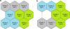 |
Fig. 1 Maps of the SOM partitioning according to sampling months (subfigure a on the left) and variables monitored (subfigure b on the right). In both cases, the k-means partitioning divided the SOM into three groups/clusters indicated with different colours and numbers. For detailed lists of dates/variables clustered in each cell see Appendices 1 and 2. |
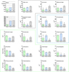 |
Fig. 2 Variables which differed across the three groups formed by the SOM. Statistically significant (p < 0.05) difference between the groups is indicated with different letters a, b, and c. The groups which did not differ from each other are marked with the same letter. Variables are arranged and separated with lines from each other so that they correspond to the SOM groups which in turn are indicated with different colours (green, blue, and grey). In the SOM component planes (small figures representing the variables monitored), colours refer to the adjacent scale bar. |
3.2 Data partitioning according to 27 study variables
Size of the optimal SOM was a 3 × 3 lattice having a quantization error of 2.394 and a topographic error of 0. The k-means partitioning divided the SOM into three clusters with CH of 9.382 (Fig. 1). In Figure 3, the 27 variables have been arranged in three clusters according to the second step SOM and associated with the groups from the first step SOM.
The first cluster was the largest. It consisted of 12 variables indicating primary production and nutrients together with diatoms, three groups of flagellates (Dinophyceae, Choanoflagellata, and Raphidophyceae), and protozoa. These variables had their highest values in samples which associated to the “1990s group” in the first step SOM (green colour in Fig. 3).
The second cluster was comprised of water temperature and precipitation together with cyanobacteria, three groups of algae (Chrysophyceae, Chlorophyceae, and Cryptophyceae), rotifers, and crustacean zooplankton. These variables had their highest values in samples which associated to the “summer group” in the first step SOM (blue colour in Fig. 3).
The third cluster was the smallest. It consisted of discharge together with five physical and chemical variables (water colour, concentrations of dissolved organic and inorganic carbon, ammonium, and nitrite and nitrate N), but no biological variables. These six variables had their highest values in samples, which associated to the “autumn group” in the first step SOM (grey colour in Fig. 3).
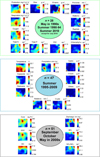 |
Fig. 3 Associations between the groups from the first step SOM and clusters from the second step SOM. The first SOM divided the data into three groups according to months and years of sampling. The second SOM divided the data into three clusters according to 27 variables monitored. In the figure, the groups are indicated with different colours (green, blue, and grey) and the variables are situated close to the group to which they associated with. n refers to the number of sampling dates per group. |
3.3 Trends in time series
Annual variation was large in all variables and a major proportion of the variables, 22 out of 27 (81%), showed no long-term trend. Water temperature, colour, DOC, nitrite-nitrate N, and chrysophytes showed an increasing monotonic trend in contrast to DO, choanoflagellates, and cladocerans which showed a decreasing monotonic trend (Fig. 4). Among the physical and chemical variables the trend was most obvious in the average level of water colour which increased from c. 100 to over 160 mg Pt L−1 within 15 years. Interestingly, the average level of DO decreased rather linearly until 2006, when the direction of the trend changed. A remarkable hundredfold decrease in the density of choanoflagellates seems linear but due to the lack of samples between 1998 and 2003 the possibility of a sudden fall in the density cannot be completely ruled out.
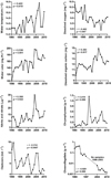 |
Fig. 4 Variables which showed increasing or decreasing trends according to the Mann–Kendall test. Note the logarithmic-scale of y-axis in the case of Choanoflagellata. |
3.4 Additional SOM including also incomplete wintertime data
The SOM map resulted was unsatisfactory (Appendix 3). Nearly all statistical units; in this case, sampling dates, with incomplete data clustered into three out of 25 best-matching units. This denotes that missing values guided data partitioning, which, obviously, concealed genuine associations across the sampling dates. Moreover, quantization and topographic errors suggested several optimal sizes for the SOM, which is a sign of low SOM quality (Vesanto et al., 2000).
The additional SOM clustered nearly all complete wintertime data into three cells including no data collected during ice-free periods (Appendix 3), which means that this SOM was unable to add new information to results of the two main SOMs.
4 Discussion
In general, the SOM method offers flexible and versatile possibilities to cluster large data sets. Typically, the abilities of SOM to detect both spatial and temporal phenomena simultaneously (Astel et al., 2007) and associate clusters based on spatial or temporal sampling points with those based on variables measured (Voutilainen et al., 2012) are highlighted. In this study, the SOM method clustered the whole data into three major categories of which the first one consisted of variables with high concentration, biomass and/or abundance in spring during 1990s, or during the first five summer seasons and summer 2010. The variables of this category included the metabolic processes, DO, total-N, total-P, chlorophyll a, and taxonomical groups of plankton known to exist in spring (Dinophyceae and ciliates). Also Gonyostomum semen, a migratory Raphidophycean algal species with very high late summer biomass during the first few years was grouped into that category. The second category consisted of all other zooplankton taxonomical groups, i.e. except ciliate protozoans, and cyanobacteria together with three major groups of phytoplankton, Chlorophyceae, Cryptophyceae, and Chrysophyceae. The abiotic factors belonging to this category were water temperature and precipitation. The common season of this category was summer. The third category included colour, DOC, DIC, ammonium, and nitrite-nitrate, as well as discharge, and the season was clearly autumn or spring, during the last 12 years (1999–2010), thus the period when the water column was unstratified.
The categories grouped by the SOM seemed logical because the different seasons clearly had their own specific abiotic conditions and plankton organisms. This finding is in accordance with our previous analyses (Arvola et al., 2014; Vuorenmaa et al., 2014). It also makes sense that the SOM separated the first few summer seasons of 1990s from the rest. The reason for this separation is that at the beginning of 1990s the lake was more productive than later on, indicated by higher primary production, chlorophyll a concentration, and biomass values in 1990–1995 compared to those taken afterwards (Arvola et al., 2014). However, based on our knowledge of the lake it was a surprise that spring and summer seasons were grouped together by the SOM. One possible explanation is the change in sampling regime that occurred. During the first seven years (1990–1996), the annual sampling program was started in January and continued until May but since 1997 regular sampling started only after the lake became ice-free. In some years, this occurred in April but in others, the lake was not ice-free until the middle of May. This may muddle the calculations because sometimes there were very high phytoplankton biomasses already under the ice in April. The additional SOM including also incomplete data collected in winter; however, did not support this explanation. The additional SOM instead clearly separated wintertime data from data collected during ice-free periods. In our previous data analyses (Arvola et al., 2014; Lehtovaara et al., 2014; Vuorenmaa et al., 2014), we did not focus on the period before ice-out, and due to differences in the ice break-up time between the years we considered that the onset of the “annual season” started on week 20.
The second category consisted of several phytoplankton groups which do not necessarily produce a huge biomass in the lake but are seemingly important food for metazooplankton, also included in this category. Therefore, category two makes sense regarding the ecosystem function. Water temperature was also included in this category which somehow underlines that it might be a period with intense grazing and rapid nutrient turnover. The third category associated water chemistry variables which all are linked to the inflow from the catchment (colour, DOC) and/or the water column mixing (ammonium-N, DIC).
Similar colour distributions within each category in Figure 3 indicate interactions between the variables. For example, in category one, chlorophyll a and the biomass of G. semen had a rather identical distribution. Total P had almost identical distribution with chlorophyll a and G. semen while primary production and the biomass of Dinophyceae and G. semen overlapped. In category two, copepods and cyanobacteria as well as chrysophytes overlapped, and in category three, the dissolved fractions of N, DOC, colour, and discharge, suggesting that ammonium and nitrate were transported from the catchment to the lake rather than from deeper water layers up to the surface.
The long-term trends detected by the Mann–Kendall test were in good accordance with our previous analyses (Arvola et al., 2014; Lehtovaara et al., 2014; Vuorenmaa et al., 2014), which increases reliability of the present results. The trends indicated an increase in water temperature, nitrite-nitrate N concentration, and DOC, and, respectively, a decrease in DO concentration.
From the perspective of global change, eutrophication, climate warming, as well as restoration and management of lakes and reservoirs it is highly important to detect these trends so that they can be used as a starting point when predicting the future of aquatic environments and water resources (O'Reilly et al., 2015). Although the SOM logically clustered the data according to temporal sampling points, detecting temporal trends solely on the basis of the SOM would have been unsure. Modifications of the SOM (Barreto, 2007) as well as combinations of the SOM and other techniques (Lin and Chen, 2005) have been successfully applied to time series forecasting, but the basic unsupervised SOM is not the solution when the purpose is to search for temporal trends (see also Voutilainen et al., 2012).
5 Conclusions
Although processes and interactions between the variables cannot be analysed in detail by the SOM, it provides a useful method for grouping the variables of such a large multi-dimensional data set. Even though other analytical tools together with the SOM may provide new options for the analysis, it remains that long-term ecological data sets may be difficult to analyse thoroughly without any supporting experimental results. Therefore, a good strategy for understanding complex processes and inter-actions is to, whenever possible, use different approaches in how studies are performed (field vs. experimental) and employing a variety of analytical tools.
Based on the present study, sampling should minimize the number of missing values. Even flexible statistical techniques, such as SOM, are vulnerable to biased results due to incomplete data. If monthly sampling is not possible, researchers should consider a less frequent but complete sampling. We do not recommend replacing missing values with means, for example, because it unintentionally reduces dimensionality and may even cause misleading results, if conclusions regarding associations across variables base on values of which some are measured and some approximated according to the measured values.
Taking samples also during wintertime, when boreal lakes are less active due to low temperature and amounts of sunlight, is important for detecting long-term trends. Differences between winter and summer, in general, tend to be larger than differences between adjacent years, which means that drawing conclusions on wintertime is not possible based on summertime data.
Acknowledgements
We thank Lammi Biological Station, University of Helsinki, for providing the long-term data sets and other support during the study. The monitoring at Valkea-Kotinen has been supported by the Academy of Finland through several projects (FOOD CHAINS, METHANO, TRANSCARBO, PRO-DOC), the Ministry of Environment (1990–1996), EURO-LIMPACS EU-project, and the Lammi Biological Station, University of Helsinki. We also thank John Loehr for the English corrections and comments on the manuscript.
Appendices
Distribution of sampling months into cells of SOM groups.
Distribution of study variables into cells of SOM clusters.
Results of SOM including also incomplete data collected in winter, 1990–2010.
References
- Adrian R, Deneke R. 1996. Possible impact of mild winters on zooplankton succession in eutrophic lakes of the Atlantic European area. Freshw Biol 36: 757–770. [CrossRef] [Google Scholar]
- Arvola L, Salonen K, Keskitalo J, Tulonen T, Järvinen M, Huotari J. 2014. Plankton metabolism and sedimentation in a small boreal lake – a long-term perspective. Boreal Environ Res 19A: 83–96. [Google Scholar]
- Astel A, Tsakovski S, Barbieri P, Simeonov V. 2007. Comparison of self-organizing maps classification approach with cluster and principal components analysis for large environmental data sets. Water Res 41: 4566–4578. [Google Scholar]
- Barreto GA. 2007. Time series prediction with the self-organizing map: a review. In: Hammer B, Hitzler P, eds. Perspectives of neural-symbolic integration. Volume 77 of the series Studies in Computational Intelligence. Berlin: Springer-Verlag, pp. 135–158. [Google Scholar]
- Beisner BE, Peres-Neto PR, Lindström ES, Barnett A, Longhi ML. 2006. The role of environmental and spatial processes in structuring lake communities from bacteria to fish. Ecology 87: 2985–2991. [CrossRef] [PubMed] [Google Scholar]
- Borcard D, Gillet F, Legendre P. 2011. Numerical ecology with R. New York: Springer, 306 p. [EDP Sciences] [Google Scholar]
- Calinski T, Harabasz J. 1974. A dendrite method for cluster analysis. Commun Stat 3: 1–27. [Google Scholar]
- Compin A, Céréghino R. 2007. Spatial patterns of macroinvertebrate functional feeding groups in streams in relation to physical variables and land-cover in Southwestern France. Landsc Ecol 22: 1215–1225. [CrossRef] [Google Scholar]
- Forsius M, Ahonen J, Alveteg M, et al. 1998. Model interaction for the assessment of emission scenarios. In: Forsius M, Guardans R, Jenkins A, Lundin L, Nielsen KE, eds. Integrated monitoring: environmental assessment through model and empirical analysis. Final results from the EU/Life-Project Development of Assessment and Monitoring Techniques at Integrated Monitoring Sites in Europe. The Finnish Environment 218. Helsinki: Finnish Environment Institute, pp. 92–99. [Google Scholar]
- Futter MN, Forsius M, Holmberg M, Starr M. 2009. A long-term simulation of the effects of acidic deposition and climate change on surface water dissolved organic carbon concentrations in a boreal catchment. Hydrol Res 40: 291–305. [CrossRef] [Google Scholar]
- Gaedke U, Schweizer A. 1993. The first decade of oligotrophication in Lake Constance. I. The response of phytoplankton biomass and cell size. Oecologia 93: 268–275. [CrossRef] [PubMed] [Google Scholar]
- Heini A, Puustinen I, Tikka M, Jokiniemi A, Leppäranta M, Arvola L. 2014. Strong dependence between phytoplankton and water chemistry in a large temperate lake: spatial and temporal perspective. Hydrobiologia 731: 139–150. [CrossRef] [Google Scholar]
- Hipel KW, McLeod AI. 1994. Time series modelling of water resources and environmental systems. In: Developments in water science, Vol. 45. Amsterdam: Elsevier, 1012 p. [Google Scholar]
- Holmberg M, Futter MN, Kotamäki N, et al. 2014. Effects of changing climate on the hydrology of a boreal catchment and lake DOC – probabilistic assessment of a dynamic model chain. Boreal Environ Res 19A: 66–82. [Google Scholar]
- Huotari J, Ojala A, Peltomaa E, Pumpanen J, Hari P, Vesala T. 2009. Temporal variations in surface water CO2 concentration in a boreal humic lake based on high frequency measurements. Boreal Environ Res 14: 48–60. [Google Scholar]
- Huttunen JT, Alm J, Liikanen A, et al. 2003. Fluxes of methane, carbon dioxide and nitrous oxide in boreal lakes and potential anthropogenic effects on the aquatic greenhouse gas emissions. Chemosphere 52: 609–621. [CrossRef] [PubMed] [Google Scholar]
- Jones RI, Grey J, Sleep D, Arvola L. 1999. Stable isotope analysis of zooplankton carbon nutrition in humic lakes. Oikos 86: 97–104. [CrossRef] [Google Scholar]
- Jylhä K, Laapas M, Ruosteenoja K, et al. 2014. Climate variability and trends in the Valkea-Kotinen region, southern Finland: comparisons between the past, current and projected climates. Boreal Environ Res 19A: 4–30. [Google Scholar]
- Kalteh AM, Hjorth P, Berndtsson R. 2008. Review of the self-organizing map (SOM) approach in water resources: analysis, modelling and application. Environ Modell Softw 23: 835–845. [Google Scholar]
- Kangur K, Park Y-S, Kangur A, Kangur P, Lek S. 2007. Patterning long-term changes of fish community in large shallow Lake Peipsi. Ecol Model 203: 34–44. [CrossRef] [Google Scholar]
- Keskitalo J, Salonen K. 1998. Fluctuations of phytoplankton production and chlorophyll concentrations in a small humic lake during six years (1990–1995). In: George DG, Jones JG, Punčochář P, Reynolds CS, Sutcliffe DW, eds. Management of lakes and reservoirs during global climate change. Dordrecht: Kluwer Academic Publishers, pp. 93–109. [CrossRef] [Google Scholar]
- Kohonen T. 1990. The self-organizing map. P IEEE 78: 1464–1480. [CrossRef] [Google Scholar]
- Kohonen T. 2013. Essentials of the self-organizing map. Neural Netw 37: 52–65. [CrossRef] [PubMed] [Google Scholar]
- Kurka A-M, Starr M. 2014. Relationship between decomposition of cellulose in the soil and tree stand characteristics in natural boreal forests. Plant Soil 197: 1677–1675. [Google Scholar]
- Lehtovaara A, Arvola L, Keskitalo J, et al. 2014. Responses of zooplankton to long-term environmental changes in a small boreal lake. Boreal Environ Res 19A: 97–111. [Google Scholar]
- Lin G-F, Chen L-H. 2005. Time series forecasting by combining the radial basis function network and the self-organizing map. Hydrol Process 19: 1925–1937. [CrossRef] [Google Scholar]
- Magnuson JJ, Benson BJ, Kratz TK. 2004. Patterns of coherent dynamics within and between lake districts at local to intercontinental scales. Boreal Environ Res 9: 359–369. [Google Scholar]
- Magnuson JJ, Kratz TK, Benson BJ, Webster KE. 2006. Coherent dynamics among lakes. In: Magnuson JJ, Kratz TK, Benson BJ, eds. Long-term dynamics of lakes in the landscape: long-term ecological research on north temperate lakes. New York: Oxford University Press, pp. 89–106. [Google Scholar]
- Oja M, Kaski S, Kohonen T. 2002. Bibliography of Self-Organizing Map (SOM) papers: 1998–2001 addendum. Neural Comput Surv 3: 1–156. [Google Scholar]
- O'Reilly C, Sharma S, Gray DK, et al. 2015. Rapid and highly variable warming of lake surface waters around the globe. Geophys Res Lett 42: 10773–10781. [CrossRef] [Google Scholar]
- Park Y-S, Céréghino R, Compin A, Lek S. 2003. Applications of artificial neural networks for patterning and predicting aquatic insect species richness in running waters. Ecol Model 160: 265–280. [CrossRef] [Google Scholar]
- Peltomaa E, Ojala A. 2010. Size-related photosynthesis of algae in a strongly stratified humic lake. J Plankton Res 32: 341–355. [CrossRef] [Google Scholar]
- Peltomaa E, Ojala A, Holopainen A-L, Salonen K. 2013a. Changes in phytoplankton in a boreal lake during a 14-year period. Boreal Environ Res 18: 387–400. [Google Scholar]
- Peltomaa E, Zingel P, Ojala A. 2013b. Weak response of the microbial food web of a boreal humic lake to hypolimnetic anoxia. Aquat Microb Ecol 68: 91–105. [CrossRef] [Google Scholar]
- Pölzlbauer G, Dittenbach M, Rauber A. 2006. Advanced visualization of Self-Organizing Maps with vector fields. Neural Netw 19: 911–922. [CrossRef] [PubMed] [Google Scholar]
- Rask M, Sairanen S, Vesala S, Arvola L, Estlander S, Olin M. 2014. Population dynamics and growth of perch in a small, humic lake over a 20-year period – importance of abiotic and biotic factors. Boreal Environ Res 19A: 112–123. [Google Scholar]
- Rimet F, Druart J-C, Anneville O. 2009. Exploring the dynamics of plankton diatom communities in Lake Geneva using emergent self-organizing maps (1974–2007). Ecol Inform 4: 99–110. [CrossRef] [Google Scholar]
- Ruoho-Airola T, Hatakka T, Kyllönen K, Makkonen U, Porvari P. 2014. Temporal trends in the bulk deposition and atmospheric concentration of acidifying compounds and trace elements in the Finnish Integrated Monitoring catchment Valkea-Kotinen during 1988–2011. Boreal Environ Res 19A: 31–46. [Google Scholar]
- Salonen K, Arvola L, Tulonen T, et al. 1992a. Planktonic food chains of a highly humic lake. I. A mesocosm experiment during the spring primary production maximum. Hydrobiologia 229: 125–142. [CrossRef] [Google Scholar]
- Salonen K, Kankaala P, Tulonen T, et al. 1992b. Planktonic food chains of a highly humic lake. II. A mesocosm experiment in summer during dominance of heterotrophic processes. Hydrobiologia 229: 143–157. [CrossRef] [Google Scholar]
- Saloranta T, Forsius M, Järvinen M, Arvola L. 2009. Impacts of projected climate change on the thermodynamics of a shallow and deep lake in Finland: model simulations and Bayesian uncertainty analysis. Hydrol Res 40: 234–247. [CrossRef] [Google Scholar]
- Samad T, Harp SA. 1992. Self-organization with partial data. Network 3: 205–212. [CrossRef] [Google Scholar]
- Sathya R, Abraham A. 2013. Comparison of supervised and unsupervised learning algorithms for pattern classification. IJARAI 2: 34–38. [Google Scholar]
- Siegel S, Castellan NJ Jr. 1988. Nonparametric statistics for the behavioural sciences. Singapore: McGraw-Hill Book Company, 399 p. [Google Scholar]
- Starr M, Ukonmaanaho L. 2004. Results from the first round of the integrated monitoring soil chemistry subprogramme. In: Ukonmaanaho L, Raitio H, eds. Forest condition in Finland. National report 2000. Research papers 824. Helsinki: Finnish Forest Research Institute, pp. 140–157. [Google Scholar]
- Vesanto J. 1999. SOM-based data visualization methods. Intell Data Anal 3: 111–126. [CrossRef] [Google Scholar]
- Vesanto J, Alhoniemi E. 2000. Clustering of the self-organizing map. IEEE Trans Neural Netw 11: 586–600. [Google Scholar]
- Vesanto J, Himberg J, Alhoniemi E, Parhankangas J. 2000. SOM toolbox for Matlab 5. SOM toolbox team, report A57. Helsinki: Helsinki University of Technology, 59 p. [Google Scholar]
- Vilibić I, Mihanović H, Šepić J, Matijević S. 2011. Using Self-Organising Maps to investigate long-term changes in deep Adriatic water patterns. Cont Shelf Res 31: 695–711. [CrossRef] [Google Scholar]
- Voutilainen A, Huuskonen H. 2010. Long-term changes in the water quality and fish community of a large boreal lake affected by rising water temperatures and nutrient-rich sewage discharges – with special emphasis on the European perch. Knowl Manag Aquat Ecosyst 397: 03. [CrossRef] [EDP Sciences] [Google Scholar]
- Voutilainen A, Rahkola-Sorsa M, Parviainen J, Huttunen MJ, Viljanen M. 2012. Analysing a large dataset on long-term monitoring of water quality and plankton with the SOM clustering. Knowl Manag Aquat Ecosyst 406: 04. [CrossRef] [EDP Sciences] [Google Scholar]
- Voutilainen A, Kvist T, Sherwood PR, Vehviläinen-Julkunen K. 2014. A new look at patient satisfaction: learning from self-organizing maps. Nurs Res 63: 333–345. [CrossRef] [PubMed] [Google Scholar]
- Voutilainen A, Hartikainen S, Sherwood PR, Taipale H, Tolppanen A-M, Vehviläinen-Julkunen K. 2015. Associations across spatial patterns of disease incidences, socio-demographics, and land use in Finland 1991–2010. Scand J Public Health 43: 356–363. [CrossRef] [PubMed] [Google Scholar]
- Vuorenmaa J, Salonen K, Arvola L, Mannio J, Rask M, Horppila P. 2014. Water quality of a small headwater lake reflects long-term variations in deposition, climate and in-lake processes. Boreal Environ Res 19A: 47–65. [Google Scholar]
- Vähätalo AV, Salonen K, Münster U, Järvinen M, Wetzel RG. 2003. Photochemical transformation of allochthonous organic matter provides bioavailable nutrients in a humic lake. Arch Hydrobiol 156: 287–314. [CrossRef] [Google Scholar]
Cite this article as: Voutilainen A, Arvola L. 2017. SOM clustering of 21-year data of a small pristine boreal lake. Knowl. Manag. Aquat. Ecosyst., 418, 36.
All Tables
Variables monitored; n – total number of samples taken from May to October 1990–2010.
All Figures
|
Fig. 1 Maps of the SOM partitioning according to sampling months (subfigure a on the left) and variables monitored (subfigure b on the right). In both cases, the k-means partitioning divided the SOM into three groups/clusters indicated with different colours and numbers. For detailed lists of dates/variables clustered in each cell see Appendices 1 and 2. |
| In the text | |
|
Fig. 2 Variables which differed across the three groups formed by the SOM. Statistically significant (p < 0.05) difference between the groups is indicated with different letters a, b, and c. The groups which did not differ from each other are marked with the same letter. Variables are arranged and separated with lines from each other so that they correspond to the SOM groups which in turn are indicated with different colours (green, blue, and grey). In the SOM component planes (small figures representing the variables monitored), colours refer to the adjacent scale bar. |
| In the text | |
|
Fig. 3 Associations between the groups from the first step SOM and clusters from the second step SOM. The first SOM divided the data into three groups according to months and years of sampling. The second SOM divided the data into three clusters according to 27 variables monitored. In the figure, the groups are indicated with different colours (green, blue, and grey) and the variables are situated close to the group to which they associated with. n refers to the number of sampling dates per group. |
| In the text | |
|
Fig. 4 Variables which showed increasing or decreasing trends according to the Mann–Kendall test. Note the logarithmic-scale of y-axis in the case of Choanoflagellata. |
| In the text | |
Current usage metrics show cumulative count of Article Views (full-text article views including HTML views, PDF and ePub downloads, according to the available data) and Abstracts Views on Vision4Press platform.
Data correspond to usage on the plateform after 2015. The current usage metrics is available 48-96 hours after online publication and is updated daily on week days.
Initial download of the metrics may take a while.